Bifurcations in four-dimensional switched systems

Abstract

In this paper, the focus is on a bifurcation of period-$\mathcal{K}$ orbit that can occur in a class of Filippov-type four-dimensional homogenous linear switched systems. We introduce a theoretical framework for analyzing the generalized Poincaré map corresponding to switching manifold. This provides an approach to capturing the possible results concerning the existence of a period-$\mathcal{K}$ orbit, stability, a number of invariant cones, and related bifurcation phenomena. Moreover, the analysis identifies criteria for the existence of multi-sliding bifurcation depending on the sensitivity of the system behavior with respect to changes in parameters. Our results show that a period-two orbit involves multi-sliding bifurcation from a period-one orbit. Further, the existence of invariant torus, crossing-sliding, and grazing-sliding bifurcation is investigated. Numerical simulations are carried out to illustrate the results.

1 Introduction

Higher dimensional systems ($n > 3$) are of great significance for applications as modeling problems often require higher dimensions. Therefore, this paper aims to investigate the existence of a period-$\mathcal{K}$ orbit, multiple periodic orbits, and related bifurcation in a linear homogeneous switching system which are quite different from those in a smooth system. These phenomena and bifurcation theory are extremely important in understanding the qualitative change in the dynamical behavior that appears on the surface of discontinuity. In smooth systems these topics are especially important phenomena which exist only in the behavior of nonlinear systems and are closely related to system stability and may lead to more complicated behavior such as chaos. As an example of the existence of multiple periodic orbits, a subcritical Hopf bifurcation leads to multiple periodic orbits in a stage structured population model [23]. Moreover, in a smooth system the necessary methods have been developed, essentially based on the fact that smooth (differentiable) systems can locally be approximated by linearized systems. Key ingredients developed within that approach are the concepts of invariant manifolds, attractors, and a characterization by characteristic numbers such as Lyapunov exponents. For instance, in the context of bifurcations of equilibria and stability analysis, center manifold theory is a well-established and mathematically proven procedure to reduce the dimension of dynamical systems.

Switched dynamical system (SDS for short) exhibits a wide variety of complex phenomena which cannot be dealt with by the classical theory, but are typically observed in many models of real systems; for instance, stick-slip, chattering, grazing-sliding, and jump phenomena were observed in an automotive brake system, impact contact model of a church bell, electronic switches, and genetic networks, respectively. For historical overviews and references, see [3, 5, 6, 10, 17, 18, 22].

In addition, SDS provides a set of possible candidates for motion of transversal crossing or attractive sliding. These systems can exhibit a wide range of nonlinear phenomena including either classical bifurcations and chaos or unique phenomena, termed discontinuity-induced bifurcations, that involve the interaction of the systems’ invariant sets with the discontinuity boundaries.

Further, many researchers have used fractional differential equations to develop mathematical models that appeared in different areas of sciences. In addition, several different control methods have been applied to synchronize the fractional order chaotic systems, for instance, see [8, 9]. These results motivated us to combine the fractional differential equations and certain types of discontinuities in vector fields as a future direction of the current work.

Nowadays, there has been growing interest in the fact that the richness of dynamical behavior found in linear SDS covers almost all types of bifurcations found in nonlinear smooth systems such as limit cycles, period-doubling, chaotic transients, homoclinic and heteroclinic, and strange attractors. Furthermore, it has been pointed out that linear SDS can undergo a complex behavior and a great number of completely new bifurcations since the characteristics of these bifurcations depend critically on both the class of SDSs and the geometry of the involved boundaries. Recently, in [12] it was shown that the existence of a novel bifurcation depends sensitively on the location of the return flow. Such an example is the existence of an invariant cone for linear SDS which may exhibit that a periodic orbit will be destroyed suddenly without any change in its stability. Further, in [19] it was shown that the planar linear SDS which has no equilibria in each subsystem, neither real nor virtual, can exhibit at least one limit cycle. For a review of the available results, see [3, 4, 6, 7, 12, 14, 19, 21, 27]. According to these researchers, we note that the current results of bifurcation theory for SDS are still incomplete and scarce. What is more, there is no general classification strategy proposed due to the lack of smoothness, suitable methods, and techniques.

Our approach (in collaboration with Küpper and Weiss, see [12, 15, 16, 18, 25, 26]) is linked with the existence of invariant surfaces in the phase space which is separated by a discontinuity manifold. It has been shown that the existence of invariant cones for SDS plays a central role in understanding the often complicated dynamical behavior near fixed points. The investigation of the dynamical behavior of the original problem is reduced to the dynamics on a two-dimensional invariant surface, carrying the essential dynamics and stability analysis of the full system. Further, we have shown how the dynamics of sliding flow can be achieved by using a generalized notion of the existence of invariant cones when the sliding motion takes place on the switching surface. Here the notion of an invariant cone appeared generalizing the focus to an object on a cone consisting of periodic orbits or orbits spiraling “in” and “out” of zero, respectively. This approach allows us to prove the existence of some sliding bifurcations for a class of linear SDSs related to invariant cones. This approach has been generalized to nonlinear SDSs in two possible behaviors: transversal crossing and attractive sliding mode. Starting with a piecewise linear system as basic system, it has been shown that the corresponding invariant cones will be deformed to a cone-like surface if higher order terms are added. In that way, we have established a similar reduction procedure to a lower dimensional system for nonlinear SDSs as has been achieved for a smooth system via the center manifold approach.

One method of studying SDS is by constructing a suitable generalized Poincaré map which has several useful properties [16] and then studying its dynamics. Therefore, the existence of invariant cones is equivalent to the existence of positive real eigenvalues of the return Poincaré map.

In this paper, we extend this approach to investigate the existence of the period-$\mathcal{K}$ orbit, a number of invariant cones, and associated phenomena. We identify three main challenges associated with finding period-$\mathcal{K}$ orbit (i.e., orbits intersecting the surface of discontinuity $\mathcal{K}$ times). The first is to find the lowest positive times of intersection with the switching surface that are dependent on ξ in a nonlinear way. The second is to construct a Poincaré map analytically, which is not an easy task. The third is to find an eigenvector which forms the period- $\mathcal{K}$ orbit.

One further aim of this work is to investigate the existence of multi-sliding, sliding bifurcation, and dynamics around period-$\mathcal{K}$ orbit (i.e., invariant torus). In this situation the trajectories come back to the switching surface several times before close the orbit under the Poincaré map. The main results are formulated in Theorem 1.

The contribution of this work is in the theory of discontinuous systems, particularly in the case of Filippov-type flow. More specifically, we obtain crossing-sliding, grazing-sliding, multiple periodic orbits, invariant cones, and their stability of a class of four-dimensional switched systems. Further, this work provides novel results concerning the existence of a period-$\mathcal{K}$ orbit with sliding mode, which is quite different from what is known for a three-dimensional system with single discontinuity surface.

Let us start with a simple example in order to show that the basic reason for the existence of period-doubling bifurcation is the presence of certain types of nonlinearities in SDS.

2 Model of the vibration system excited by a harmonic force

We consider a simple vibration system of a single-degree-of-freedom oscillator with a bilinear restoring force [22]. When the system is externally excited by a harmonic force, the equation of motion may be written as follows:

$$ \begin{aligned} &\ddot{x}+2 \alpha \dot{x}+x=\beta \cos(wt),\quad \mbox{for } x\leq x_{0}, \\ &\ddot{x}+2 \alpha \dot{x}+\bar{w}^{2}+ \bigl(1-\bar{w}^{2} \bigr)x_{0}=\beta \cos(wt),\quad \mbox{for }x\geq x_{0}. \end{aligned} $$

(1)

It is well known that the methods for analysis of nonlinear systems usually require a representation of the system as a set of autonomous first order ODE. To preserve the property of “nonsmoothness”, the system has to be rewritten as an autonomous system by introducing time as an additional state variable.

By letting $\xi_{1}=x$, $\xi_{2}=\dot{x}$, $\xi_{3}=w t$ ($\xi_{3}$ mod $2\pi/w$), the following system can be obtained:

$$ \begin{aligned} &\dot{\xi }= \begin{pmatrix} \xi_{2} \\ -\bar{\omega}\xi_{1}-2\alpha\xi_{2}+\beta \cos(\xi_{3})\\ \omega \end{pmatrix},\quad e_{1}^{T}\xi< 0, \\ & \dot{\xi }= \begin{pmatrix} \xi_{2} \\ -\xi_{1}-2\alpha\xi_{2}+\beta \cos(\xi_{3})\\ \omega \end{pmatrix} ,\quad e_{1}^{T}\xi>0, \end{aligned} $$

(2)

where the discontinuity surface is defined by $\mathcal {M}=\{\xi\in \mathbb {R}^{3} | e_{1}^{T}\xi=0\}$.

We note that if $\alpha=\beta=0$, then system (2) has a continuous family of periodic orbits. But if $\alpha\neq\beta\neq 0$, then a variation of the dynamical process is a transition of an orbit with period T into an orbit with period 2T. In this model the bifurcation parameter is taken as ω and the other parameters are fixed as $\bar{w}=4$, $\alpha=0.125$. The numerical simulation illustrates that the bifurcation actually occurs between $w=2.40$ and $w=2.42$. Figure 1 shows the transition of a period-one orbit to period-two orbits. This transition is called periodic doubling bifurcation which occurs due to the presence of nonlinear harmonic force.

Figure 1

Transition of a period-one orbit to period-two orbits in nonlinear system (2)

In the next section we introduce a class of four-dimensional homogenous linear SDSs with two-zone and provide a methodology to ensure that the system has a period-$\mathcal{K}$ orbit.

3 The existence of a period-${{\mathcal{K}}}$ orbit in SDS

3.1 Setting of the problem

We start our investigations by considering a four-dimensional homogenous linear SDS for which the evolution of a variable ξ in some region is determined by the equations

$$ \begin{aligned} \textstyle\begin{array}{rl} \dot{\xi_{1}}&= \lambda^{-} \xi_{1}-\xi_{2}+\mu\beta^{-}\xi_{3}+\mu(\alpha^{-}-\lambda^{-})\xi_{4},\\ \dot{\xi_{2}}&= \xi_{1}+\lambda^{-} \xi_{2}-\mu\xi_{4}, \quad \xi_{1}< 0,\\ \dot{\xi_{3}}&= \alpha^{-}\xi_{3}-\beta^{-}\xi_{4},\\ \dot{\xi_{4}}&= \beta^{-}\xi_{3}+\alpha^{-}\xi_{4}, \end{array}\displaystyle \qquad \textstyle\begin{array}{rl} \dot{\xi_{1}}&= \lambda^{+} \xi_{1}-\xi_{2},\\ \dot{\xi_{2}}&= \xi_{1}+\lambda^{+} \xi_{2}, \quad \xi_{1}>0,\\ \dot{\xi_{3}}&= \alpha^{+}\xi_{3}-\beta^{+}\xi_{4},\\ \dot{\xi_{4}}&= \beta^{+}\xi_{3}+\alpha^{+}\xi_{4}. \end{array}\displaystyle \end{aligned} $$

(3)

This has a switching surface given by $\mathcal {M}=\{\xi \in R^{4}| \xi_{1}=0\}$. At $\xi\in \mathcal {M}$, the flow can cross through or slide (attracting or repulsive) along the three-dimensional discontinuity surface. These two behaviors are classified by means of a vector field evaluation at $\mathcal {M}$. Hence, the both sets of crossing regions (see Fig. 2) are given by $\mathcal {M}^{c}_{-}=\{\xi\in \mathcal {M}| \xi_{2}>\mu(\beta^{-}\xi_{3}+(\alpha^{-}-\lambda^{-}) \xi_{4})>0\}$ and $\mathcal {M}^{c}_{+}=\{\xi\in \mathcal {M}| \xi_{2}<\mu(\beta^{-}\xi_{3}+(\alpha^{-}-\lambda^{-}) \xi_{4})<0\}$. The sliding regions are given by $\mathcal {M}^{s}_{-}=\{\xi\in \mathcal {M}| 0<\xi_{2}<\mu(\beta^{-}\xi_{3}+(\alpha^{-}-\lambda^{-}) \xi_{4})\}$ and $\mathcal {M}^{s}_{+}=\{\xi\in \mathcal {M}| 0 > \xi_{2} > \mu(\beta^{-}\xi_{3}+(\alpha^{-}-\lambda^{-}) \xi_{4})\}$, where $\mathcal {M}^{s}_{-}$ is called attractive sliding mode and $\mathcal {M}^{s}_{+}$ is called repulsive sliding mode. Further, $\mathcal {M}^{0}_{-}=\{\xi \in \mathcal {M}| \xi_{2}=\mu(\beta^{-}\xi_{3}+(\alpha^{-}-\lambda^{-}) \xi_{4}\}$, $\mathcal {M}^{0}_{+}=\{\xi \in \mathcal {M}| \xi_{2}=0\}$ define the boundaries between sliding and crossing modes, and $\mathcal {M}^{0}= \mathcal {M}^{0}_{-}\cap \mathcal {M}^{0}_{+}$ defines the intersection plane between two boundaries.

Figure 2

Schematic illustration regions of crossing and sliding boundaries

The flow in $\mathcal {M}^{s}$ itself is governed by Filippov’s extension as follows: $\dot{\xi}=q A^{+}\xi+(1-q)A^{-}\xi, q\in [0, 1]$, where $q(\xi)=\frac{e_{1}^{T}A^{-}\xi}{e_{1}^{T}(A^{-}-A^{+})\xi}$ and $A^{\pm}$ is a Jacobian linearization of (3). Therefore, we have an explicit form of the sliding vector field

$$ \dot{\xi}=A^{+}\xi-\frac{e_{1}^{T} A^{+} \xi}{e_{1}^{T}(A^{-}-A^{+})\xi} \bigl(A^{-}-A^{+} \bigr)\xi. $$

(4)

This sliding system becomes a linear system if and only if there exist vectors $x,y \in \mathbb {R}^{4}$ such that $(A^{+}-A^{-} )(I-e_{1} e_{1}^{T})=x y^{T}$ holds (see Theorem 5.3 in [18]). The choice of matrices in (3) is taken in a more general form such that system (3) exhibits a rich variety of bifurcation behaviors depending on different parameters. Thus, without loss of generality, assume that

$$ \begin{aligned} &A^{\pm}= \bigl(\mathbf{S}^{\pm}\bigr)^{-1} A_{N}^{\pm}\mathbf{S}^{\pm}, \qquad \mathbf{S}^{-}= \bigl[e_{1},e_{2},e_{3}, \mu(e_{1}+e_{4}/\mu) \bigr], \\ &\mathbf{S}^{+}=I,\qquad A_{N}^{\pm}= \begin{pmatrix} \lambda^{\pm}&-1 & 0 &0 \\ 1 & \lambda^{\pm}& 0 & 0 \\ 0 & 0 & \alpha^{\pm}&-\beta^{\pm}\\ 0 & 0 & \beta^{\pm}& \alpha^{\pm}\end{pmatrix}. \end{aligned} $$

(5)

The following lemma collects several useful properties of (3).

Lemma 1

For system (3), the following properties hold:

• Eigenvalues of $A^{\pm}$ are $\lambda^{\pm}\pm \mathbf{i}$ and $\alpha^{\pm}\pm \mathbf{i}\beta^{\pm}$ (with $\lambda^{\pm}$, $\alpha^{\pm}$, $\beta^{\pm}\in \mathbb {R}$, $\beta^{\pm}>0$).

• The origin is the only equilibrium point in each sub-system.

• The ⊕-system possesses an invariant plane $e_{3}^{T} \xi=e_{4}^{T} \xi=0$ with constant return time $t_{+}(\xi)=\pi$.

• For the ⊖-system, the surface generated by $\xi_{2}=\beta^{-} \mu \xi_{3}+\mu(\alpha^{-}-\lambda^{-}) \xi_{4}$ determines the boundary of the sliding motion area in the $(\xi_{2},\xi_{3},\xi_{4})$-phase space.

• The sliding motion is governed by linear equations if $\lambda^{+}=\lambda^{-}$, $\alpha^{+}=\alpha^{-}$, $\beta^{\pm}=0$.

• If $\mu=0$ there is no sliding motion area.

• The intersection times (hit times) are constants on rays in all regions.

• If $\xi\in \mathcal {M}^{0}$, then ξ is called a two-fold singularity or the Filippov system has a singular point.

Proof

By direct calculation of eigenvalues of $A^{\pm}$, we have $\lambda^{\pm}\pm \mathbf{i}$ and $\alpha^{\pm}\pm \mathbf{i}\beta^{\pm}$, $\beta^{\pm}>0$, and since $A^{\pm}$ are nonsingular matrices, then the origin is the only equilibrium point. For the ⊕-system, we have $\mathcal {M}^{c}_{-}=\{\xi\in \mathcal {M}|\xi_{2}>0\}$, $\mathcal {M}^{c}_{+}=\{\xi\in \mathcal {M}| \xi_{2}<0\}$; hence, the intersection time $t_{+}(\xi)=\pi$ is constant and, by means of vector field evaluation at $\mathcal {M}$, we find $\xi_{2}=\beta^{-} \mu \xi_{3}+\mu(\alpha^{-}-\lambda^{-}) \xi_{4}$ determines the boundary of the sliding motion area. In addition, let $\lambda^{+}=\lambda^{-}$, $\alpha^{+}=\alpha^{-}$, $\beta^{\pm}=0$ in (4), the sliding flow becomes linear.

Further, when $\mu=0$, we find $\mathcal {M}^{s}:=\{\phi\}$, which means that there is no sliding motion area. Furthermore, the intersection times (hit times) are constants on rays in all regions due to the homogeneity of system (3) (see [16]). Last, if $\xi\in \mathcal {M}^{0}$, we find $e_{1}^{T} A^{-}\xi=e_{1}^{T} A^{+}\xi=0$ in (4), and therefore the Filippov system has a singular point. □

Note that transformation (5) does not perturb the switching manifold $\mathcal {M}$. Then the general solution of (3) is given by

$$ \begin{aligned} \psi(t_{\pm},\xi)={}&e^{\lambda^{\pm} t_{\pm}} \bigl\{ \bigl(\cos(t_{\pm}) \bigl(\mathbf{S}^{\pm}\bigr)^{-1} e_{1}+\sin(t_{\pm}) \bigl( \mathbf{S}^{\pm}\bigr)^{-1} e_{2} \bigr)\bar{ \xi}_{1} \\ &{}+ \bigl(\cos(t_{\pm}) \bigl(\mathbf{S}^{\pm}\bigr)^{-1} e_{2}-\sin(t_{\pm}) \bigl( \mathbf{S}^{\pm}\bigr)^{-1} e_{1} \bigr)\bar{ \xi}_{2} \bigr\} \\ &{}\times e^{\alpha^{\pm} t_{\pm}} \bigl\{ \bigl(\cos \bigl(\beta^{\pm}t_{\pm} \bigr) \bigl(\mathbf{S}^{\pm}\bigr)^{-1} e_{3}+ \sin \bigl(\beta^{\pm}t_{\pm} \bigr) \bigl(\mathbf{S}^{\pm}\bigr)^{-1} e_{4} \bigr)\bar{\xi}_{3} \\ &{}+ \bigl(\cos \bigl(\beta^{\pm}t_{\pm} \bigr) \bigl( \mathbf{S}^{\pm}\bigr)^{-1} e_{4}-\sin \bigl( \beta^{\pm}t_{\pm} \bigr) \bigl(\mathbf{S}^{\pm}\bigr)^{-1} e_{3} \bigr)\bar{\xi}_{4} \bigr\} , \end{aligned} $$

(6)

where

$$ \mathbf{S}^{\pm}\xi(0) =\bar{\xi},\quad \xi(0)= \bigl(0, \xi_{2}^{0},\xi_{3}^{0}, \xi_{3}^{0} \bigr)^{T}\in \mathcal {M}^{c} . $$

The general solution (6) allows us to construct Poincaré maps $P_{\pm}$ for ⊕ and ⊖-systems, respectively. The flow starts from the initial point $\xi^{0}\in \mathcal {M}^{c}_{-}$ and spends a time $t_{-}$ before it returns to $\psi(t_{-},\xi)\in \mathcal {M}^{c}_{+}$, then we can define the map $P_{-}(\xi):= \mathcal {M}^{c}_{-} \rightarrow \mathcal {M}^{c}_{+}$. At that point, the flow starts once again and spends a time $t_{+}$ before it reaches $\psi (t_{+},\xi)\in \mathcal {M}^{c}_{-}$, we can define the map $P_{+}(\xi):= \mathcal {M}^{c}_{+} \rightarrow \mathcal {M}^{c}_{-}$. The return times $t_{\pm}(\xi)$ depend on ξ and are determined as the lowest positive root of $e^{T}_{1} \psi^{\pm}(t_{\pm},\xi)=0$. If the flow of a subsystem of (3) arrives at the attractive sliding region $\mathcal {M}^{s}_{-}$, the sliding flow can be observed along a three-dimensional discontinuity surface, where $\xi \in \mathcal {M}^{s}$, and let $t_{s}$ be the time spent in $\mathcal {M}^{s}$. Then we define the sliding map as $P_{s}:= \mathcal {M}^{s}_{-} \rightarrow \mathcal {M}^{s}_{-}$.

From a local point of view, a generalized Poincaré map can be thought of as a composition of sub-maps ($P_{-}, P_{+}, P_{s}$). Further, if the trajectories of (3) come back to $\mathcal {M}$ several times before close the orbit, then $P^{\mathcal{K}}$ represents the composition of P with itself or sub-maps $\mathcal{K}$ times.

Lemma 2

Consider a generalized Poincaré mapping $P^{\mathcal{K}}$ (where $P^{\mathcal{K}}$ is the $\mathcal{K}$th iterate of P) structure for period-$\mathcal{K}$ orbit either without sliding mode

$$\begin{aligned} \begin{aligned} &P^{\mathcal{K}}(\xi)=(P_{i}\circ P_{j})^{\mathcal{K}}(\xi)=\xi,\quad i,j\in\{+,-\}, i\neq j, \mathcal{K}>1, \\ &P^{\mathcal{K}-1}(\xi)\neq\xi\end{aligned} \end{aligned}$$

or with sliding mode

$$\begin{aligned} \begin{aligned} &P^{\mathcal{K}}(\xi)=(P_{i}\circ P_{k} \circ P_{j})^{\mathcal{K}}(\xi)=\xi,\quad i,j,k\in\{+,-,s\}, i\neq j\neq k, \mathcal{K}>1, \\ &P^{\mathcal{K}-1}(\xi)\neq\xi, \end{aligned} \end{aligned}$$

such that $t_{-}^{\mathcal{K}}, t_{+}^{\mathcal{K}}, t_{s}^{\mathcal{K}}$ exist. Then SDS (3) has a period-$\mathcal{K}$ orbit without or with sliding mode, respectively.

Proof

We assume that the local Poincaré section is $\mathcal {M}$ and the time functions $t_{\pm}^{\mathcal{K}}, t_{s}^{\mathcal{K}}$ exist. By using the fact that a periodic point of the full system (3) with crossing the Poincarè section $\mathcal{K}$ times is a fixed point of the $\mathcal {P}^{\mathcal{K}}$ iterate of $\mathcal {P}$, by cyclic invariance, SDS (3) has a period-$\mathcal{K}$ orbit without or with sliding mode. □

The existence of invariant cones for (3) depends on the existence of a positive eigenvalue of the generalized Poincaré map (i.e., $P^{\mathcal{K}}(\xi)=\mu_{c}\xi, \mu_{c}>0$). This leads to the fact that the existence of a period-$\mathcal{K}$ orbit is just a sufficient condition for the existence of invariant cone foliated by orbits.

3.2 Main results

The main results focus on the classification of the possible bifurcation scenarios that can occur in (3) and are summarized in the following theorem. This theorem provides a general framework and conditions in which the existence of period-$\mathcal{K}$ orbit, stability, a number of invariant cones, multi-sliding bifurcation, invariant torus, and crossing or grazing-sliding bifurcation in system (3) take place. These results are carried out by using the characterization of a generalized Poincaré map.

Theorem 1

For the linear SDS (3), the following statements hold:

(I):

Suppose the case $\lambda^{+}=-\lambda^{-}$. Then:

• 1. The system has a flat periodic orbit (degenerate situation) contained with the invariant plane ($\bar{\xi}_{1},\bar{\xi}_{2}$) and $t_{-}=\pi$.

• 2. Assume also that $\alpha^{-}=\lambda^{-}=-\lambda^{+}=-\alpha^{+}$, $\beta^{-}+\beta^{+}=K\in Z$, to characterize complex behaviors.

  • 2.1 When $\bar{\xi}\in \mathcal {M}^{c}_{-}$ and $\bar{\xi}_{2}>\mu \beta^{-} \bar{\xi}_{3}$. Then the system has a family of period-one orbits with period $T=2\pi$ if K is even and a family of period-two orbits with period $T=4\pi$ if K is odd such that $\beta^{+}$ is even (i.e., $\beta^{-}$ is odd). Further, if $\beta^{+}$ is odd (i.e., $\beta^{-}$ is even), then the system has three families of period-two orbits.

  • 2.2 When $\bar{\xi}\in \mathcal {M}^{0}_{-}$ and $\bar{\xi}_{2}=\mu \beta^{-} \bar{\xi}_{3}$. Then the system has two families of period-one orbits with a segment of sliding motion if K is even, and these orbits can also undergo a grazing-sliding bifurcation. As well there is a transition from period-one orbit to period-two orbit with two segments of sliding motion (multi-sliding) if K is odd.

(II):

Assume that $\bar{\xi}\in \mathcal {M}^{0}_{-}$, $\sigma=(\alpha^{-}-\lambda^{-})<0$. Then:

• 1. The system has two families, namely short and long period-one orbits generated by the boundary surface of sliding mode, such that the image of sliding periodic boundary surface under the Poincaré map is satisfied:

  $$ \frac{\beta^{-}\sin{t_{-}}-e^{\sigma t_{-}}\sin{\beta t_{-}}}{\sigma \sin{t_{-}}+\cos{t_{-}}-e^{\sigma t_{-}} \cos{\beta^{-} t_{-}}}= \frac{\beta^{-}(e^{\lambda^{+}\pi+\lambda^{-} t_{-}} \cos(t_{-})+1)}{e^{\lambda^{+}\pi+\lambda^{-} t_{-}}(\sigma\cos(t_{-})-\sin{t_{-}})+\sigma}=0. $$

• 2. The system has a family of period-one orbits generated by $\bar{\xi}\in \mathcal {M}^{0}_{-}$ with $t_{-}\in(\pi,2\pi)$ and $\beta^{\pm}=0$ if and only if

  $$ e^{\lambda^{+}\pi+\lambda^{-} t_{-}} \bigl(\sigma\cos(t_{-})-\sin{t_{-}} \bigr)+\sigma=0. $$

• 3. The system has a family of period-one orbits with sliding mode which is generated by $\bar{\xi}\in \mathcal {M}^{0}_{-}$ with $t_{-}\in(\pi,2\pi)$ and $\beta^{\pm}=0$ if and only if

  $$ e_{1}^{T} P_{-}(\bar{\xi}) < \mu \sigma e_{3}^{T} P_{-}(\bar{\xi})< 0,\quad 0< e_{1}^{T} P(\bar{\xi}) < \mu \sigma e_{3}^{T} P(\bar{\xi}). $$

Moreover, the system undergoes the crossing-sliding bifurcation due to the transition between crossing and sliding modes.

(III):

Assume that $\sigma=0$ and $\lambda^{+}=-\lambda^{-}$. Then:

• 1. There is a family of flat periodic orbits generated by the invariant $(\bar{\xi}_{1},\bar{\xi}_{2})$-plane with period $T=2\pi$.

• 2. There are two families of period-two orbits if $\beta^{-}=1$, $\alpha^{+}=-\alpha^{-}$, one of them is generated by the boundary surface of sliding region with period $T=2\pi+\sum_{i=1}^{3} t^{(i)}_{-}$ and the other is generated by any vector $\bar{\xi}\in \mathcal {M}^{c}_{-}$ with period $T=4\pi$.

• 3. There are two families of period-one orbits if $\beta^{-}=2$, $\alpha^{+}=-\alpha^{-}$, one of them is generated by $\bar{\xi}=\{\bar{\xi}\in \mathcal {M}^{0}_{-} |\bar{\xi}_{4}=0\}$ with period $T=2\pi$ and the other is generated $\bar{\xi}=\{\bar{\xi}\in \mathcal {M}^{c}_{-}|\bar{\xi}_{4}=0\}$ with period $T=2\pi$.

(IV):

Suppose that $\mu=0$ (i.e., $\mathcal {M}^{s}=\emptyset$) and $\alpha^{+}=-\alpha^{-}$. Then:

• 1. The system has two families of period-one orbits, one of them is generated by the invariant $(\bar{\xi}_{1},\bar{\xi}_{2})$-plane with period $T=2\pi$ and the other is generated by any vector $\bar{\xi}\in \mathcal {M}$ such that $\beta^{-}+\beta^{+}=K$ is even with $T=2\pi$ if $\lambda^{+}=-\lambda^{-}$. Further, there is a transition from period-one orbit to period- two orbit if K is odd.

• 2. The system has a family of period-$\mathcal{K}$ orbits or an invariant torus if and only if K is an irrational number.

The above results are tailored to the class of four-dimensional homogenous linear SDSs (3) that form a specific subclass of Filippov-type discontinuous systems [5, 21]. In the literature [4, 12, 13, 18, 26], various results are available on the existence of invariant sets (such as invariant cones, attractivity, and period-1 orbit) and their bifurcations (such as saddle-node and sliding phenomena) of a three-dimensional homogenous linear system with single discontinuity surface. Our current work covers most of these aspects and provides novel results concerning the existence of invariant sets of SDS (3). In particular, although the existing results for period-$\mathcal{K}$ orbit ($\mathcal{K}>1$) are only associated with the problems involving nonlinear or non-homogeneous operators [5, 22], we point out in this paper that the homogeneous linear four-dimensional SDS can exhibit period-$\mathcal{K}$ orbits with/without sliding mode, which is quite different from what is known for three-dimensional SDSs with single discontinuity surface. Further, in such cases we observe a sudden transition through the discontinuity manifold.

3.3 Construction of the generalized Poincaré map

For rigorous evaluation of the generalized Poincaré map, we use analytical formulas for trajectories of system (3), which are given by (6). The Poincaré map $P_{-}(\xi):= \mathcal {M}^{c}_{-} \rightarrow \mathcal {M}^{c}_{+}$ is given as follows:

$$ P_{-}(\xi)= \begin{pmatrix} e^{\lambda^{-}t_{-}}\cos(t_{-}) & 0 & -\mu e^{\lambda^{-} t_{-}}\sin(t_{-}) \\ 0 & e^{\alpha^{-}t_{-}}\cos(\beta^{-}t_{-}) &- e^{\alpha^{-}t_{-}}\sin(\beta^{-}t_{-}) \\ 0 &e^{\alpha^{-}t_{-}}\sin(\beta^{-}t_{-}) & e^{\alpha^{-}t_{-}}\cos(\beta^{-}t_{-}) \end{pmatrix} \begin{pmatrix} \xi_{2} \\ \xi_{3} \\ \xi_{4} \end{pmatrix}. $$

Note that the return time $t_{-}(\xi)$ depends on ξ in a nonlinear way, and it is actually the first one possible in $\mathcal {M}^{c}_{-}$. It means that the trajectory of ⊖-system intersects $\mathcal {M}$ transversally if we can find the smallest positive root of the following equation:

$$ F \bigl(t_{-}(\xi) \bigr)=\sin(t_{-})\xi_{2}+\mu \cos(t_{-}) \xi_{4}-\mu e^{(\alpha^{-}-\lambda^{-})t_{-}} \bigl(\sin \bigl(\beta^{-} t_{-} \bigr) \xi_{3}+\cos \bigl(\beta^{-} t_{-} \bigr) \xi_{4} \bigr)=0. $$

(7)

Further, the Poincaré map $P_{+}(\xi):= \mathcal {M}^{c}_{+} \rightarrow \mathcal {M}^{c}_{-}$ is given as follows:

$$ P_{+}(\xi)= \begin{pmatrix} -e^{\lambda^{+}\pi} & 0 & 0 \\ 0 & e^{\alpha^{+}\pi}\cos(\beta^{+}\pi) &- e^{\alpha^{+}\pi}\sin(\beta^{+}\pi) \\ 0 &e^{\alpha^{+}\pi}\sin(\beta^{+}\pi) & e^{\alpha^{+}\pi}\cos(\beta^{+}\pi) \end{pmatrix} \begin{pmatrix} \xi_{2} \\ \xi_{3} \\ \xi_{4} \end{pmatrix}. $$

We assume $\xi\in \mathcal {M}^{c}_{-}$ (hence $\xi_{2}>0$), then we get the generalized Poincaré map

$$ \begin{aligned} P&=P_{+}\circ P_{-}(\xi) \\ &=\mathbb{B}_{1} \begin{pmatrix} -\mathbb{B}_{2} \cos{(t_{-})} & 0 & \mu \mathbb{B}_{2} \sin{(t_{-})} \\ 0 & \cos{(\beta^{+} \pi+\beta^{-} t_{-})} & -\sin{(\beta^{+} \pi+\beta^{-} t_{-})} \\ 0 & \sin{(\beta^{+} \pi+\beta^{-} t_{-})} & \cos{(\beta^{+} \pi+\beta^{-} t_{-})} \end{pmatrix} \begin{pmatrix} \xi_{2} \\ \xi_{3} \\ \xi_{4} \end{pmatrix}, \end{aligned} $$

(8)

where

$$\mathbb{B}_{1}=e^{\alpha^{+} \pi+\alpha^{-} t_{-}},\quad \mbox{and}\quad \mathbb{B}_{2}=e^{(\lambda^{+} -\alpha^{+}) \pi+(\lambda^{-} -\alpha^{-}) t_{-}}. $$

The second iterate of the generalized Poincaré return map is given as follows:

$$ P^{2}(\xi)= \begin{pmatrix} \mathbb{B} & \mathbb{D} & \mathbb{E} \\ 0 & \mathbb{C} & -\mathbb{S} \\ 0 & \mathbb{S} & \mathbb{C} \end{pmatrix} \begin{pmatrix} \xi_{2} \\ \xi_{3} \\ \xi_{4} \end{pmatrix}, $$

(9)

where

$$\begin{aligned} &\mathbb{B}=e^{2\lambda^{+}\pi+\lambda^{-}(t_{-}^{(1)}+t_{-}^{(2)})}\cos{ \bigl(t_{-}^{(1)} \bigr)}\cos{ \bigl(t_{-}^{(2)} \bigr)}, \\ &\mathbb{D}=\mu e^{(\lambda^{+}+\alpha^{+})\pi+\lambda^{-}t_{-}^{(2)}+\alpha^{-} t_{-}^{(1)}}\sin{ \bigl(t_{-}^{(2)} \bigr)}\sin{ \bigl( \beta^{+} \pi+\beta^{-} t_{-}^{(1)} \bigr)} , \\ & \begin{aligned} \mathbb{E}={}&{-}\mu \bigl(e^{2\lambda^{+}\pi+\lambda^{-}(t_{-}^{(1)}+t_{-}^{(2)})}\cos{ \bigl(t_{-}^{(2)} \bigr)} \sin{ \bigl(t_{-}^{(1)} \bigr)}\\ &{}+\mu e^{(\lambda^{+}+\alpha^{+})\pi+\lambda^{-} t_{-}^{(2)}+\alpha^{+} t_{-}^{(1)}}\sin{ \bigl(t_{-}^{(2)} \bigr)}\cos{ \bigl(\beta^{+} \pi+\beta^{-} t_{-}^{(1)} \bigr)} \bigr), \end{aligned} \\ &\mathbb{C}=e^{2\alpha^{+} \pi+\alpha^{-}(t_{-}^{(1)}+t_{-}^{(2)})}\cos{ \bigl(2\beta^{+} \pi+\beta^{-} \bigl(t_{-}^{(1)}+t_{-}^{(2)} \bigr) \bigr)}, \\ &\mathbb{S}=e^{2\alpha^{+} \pi+\alpha^{-}(t_{-}^{(1)}+t_{-}^{(2)})}\sin{ \bigl(2\beta^{+} \pi+\beta^{-} \bigl(t_{-}^{(1)}+t_{-}^{(2)} \bigr) \bigr)}. \end{aligned}$$

The second return times $t_{-}^{(2)}$ is given as the smallest positive root of the following equation:

$$ \begin{aligned} F_{2} \bigl(t_{-}^{(2)}( \xi) \bigr)={}&\sin \bigl(t_{-}^{(2)} \bigr)e_{1}^{T} P( \xi)+\mu \cos \bigl(t_{-}^{(2)} \bigr)e_{3}^{T} P( \xi)- \mu e^{(\alpha^{-}-\lambda^{-})t_{-}^{(2)}} \bigl(\sin \bigl(\beta^{-} t_{-}^{(2)} \bigr)e_{2}^{T} P(\xi) \\ &{}+\cos \bigl(\beta^{-} t_{-}^{(2)} \bigr) e_{3}^{T} P( \xi) \bigr)=0. \end{aligned} $$

(10)

In the same way, we can get $\mathcal{K}$ iterate of the Poincaré map.

Lemma 3

We assume that ξ̄ is a fixed point of the generalized Poincaré map $P(\bar{\xi})=\bar{\xi}$ or $P^{2}(\bar{\xi})=\bar{\xi}$, respectively. If all eigenvalues of linearized P (resp. $P^{2}$)) at ξ̄ satisfy $|\mu_{c}|<1$ (resp. $|\hat{\mu_{c}}|<1$), then ξ̄ is asymptotically stable, and if $|\mu_{c}|>1$ (resp. $|\hat{\mu_{c}}|>1$), then ξ̄ is unstable. If $|\mu_{c}|=1$ (resp. $|\hat{\mu_{c}}|=1$), then ξ̄ generates a periodic behavior.

If $\mathcal{K}=2$, the eigenvalues of the linearized Poincaré map (8) and (9), respectively, are given as:

$$\begin{aligned} &\mu_{c}^{1}=-\mathbb{B}_{1}\mathbb{B}_{2} \cos \bigl(t_{-}^{(1)} \bigr),\qquad \mu_{c}^{(2,3)}= \mathbb{B}_{1} \bigl(\cos \bigl(\beta^{+}\pi+\beta^{-} t_{-}^{(1)} \bigr)\pm \mathbf{i}\sin \bigl(\beta^{+}\pi+\beta^{-} t_{-}^{(1)} \bigr) \bigr), \\ &\hat{\mu}_{c}^{1}=\mathbb{B},\qquad \hat{ \mu}_{c}^{(2,3)}=\mathbb{C}\pm \mathbf{i}\mathbb{S}. \end{aligned}$$

This lemma is true if ξ̄ is a fixed point of $P^{\mathcal{K}}(\bar{\xi})$ which guarantees and determines the existence of periodic behavior and stability of system (3). Now, we are ready to prove all items of Theorem 1, respectively.

3.4 Proof of the main results

(I) Because $\bar{\xi}\in \mathcal {M}^{c}_{-}$, then the result $\bar{\xi}_{2}>\mu \beta^{-} \bar{\xi}_{3}$ directly follows from the definition of the crossing region $\mathcal {M}^{c}_{-}$. Let $\mu_{c}^{1}=1$ corresponding to a period-one orbit of the Poincaré map (8). Then we get one possible solution $\lambda^{-}=-\lambda^{+}$ and $t_{-}=\pi$ that must be verified by the nonlinear equation (7). Hence, we get

$$ F(\pi)=-\mu \xi_{4}-\mu e^{(\alpha^{-}-\lambda^{-})\pi} \bigl(\sin \bigl(\beta^{-} \pi \bigr)\xi_{3}+\cos \bigl(\beta^{-} \pi \bigr) \xi_{4} \bigr)=0. $$

(11)

If $\beta^{-}$ is odd, then we get $e^{(\alpha^{-}-\lambda^{-})\pi}=1$, which leads to $\alpha^{-}=\lambda^{-}$; and if $\beta^{-}$ is even, then we get $e^{(\alpha^{-}-\lambda^{-})\pi}=-1$, which is not possible. Moreover, regarding Lemma 2, the corresponding eigenvector, which is responsible for generating a period-one orbit, requires either $\xi_{3}=\xi_{4}=0$ or $\xi_{3}\neq 0, \xi_{4}\neq 0$.

• (a) If $\xi_{3}=\xi_{4}=0$ is invariant surface, then we obtain a flat period-one orbit contained with the invariant plane $(\bar{\xi}_{1},\bar{\xi}_{2})$, which is a trivial situation for our purposes.

• (b) If $\xi_{3}\neq 0, \xi_{4}\neq 0$ lead to $\alpha^{-}=-\alpha^{+}$ and $\beta^{-}+\beta^{+}=K\in Z$ is even. Therefore we get a nontrivial period-one orbit spanned by $\bar{\xi}\in \mathcal {M}^{c}_{-}$. For an example to show this situation where $\alpha^{-}=\lambda^{-}=-\lambda^{+}=-\alpha^{+}$ and $\beta^{-}+\beta^{+}=K\in Z$ is even, see Fig. 3(a).

  Figure 3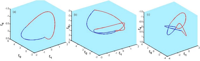

  

  (a) Nontrivial period-one orbit when $\beta^{-}=\beta^{+}=-\alpha^{-}=1$ (K is even). (b), (c) Period-two orbits when $\beta^{-}=0.5\beta^{+}=-\alpha^{-}=1$ (K is odd)

On the other hand, the existence of a period-two orbit is associated with an eigenvalue of the Jacobian of the Poincaré map (8) equal −1 and $P^{2}(\bar{\xi})=\bar{\xi}$ (Lemma 3). Then, when $\alpha^{-}=\lambda^{-}=-\lambda^{+}=-\alpha^{+}$, we find that the positive roots $t_{-}^{(1)}=t_{-}^{(2)}=\pi$ satisfy equations (7) and (10) if and only if $\beta^{-}$ is odd where $\beta^{-}+\beta^{+}=K\in Z$ is odd (i.e., $\beta^{+}$ is even). For instance, see Fig. 3(b), (c).

If $\beta^{-}$ is even (i.e., $\beta^{+}$ is odd), the three families of period-two orbits are made up for by compensatory changes in the time spent in the ⊖-system. Hence, we compute the possible intersection times under attraction of $P^{\mathcal{K}}$. Then there are three cases of existence of the intersections times that are given by (7) and (10); if $t_{-}^{(1)}\neq t_{-}^{(2)}\neq \pi$, so there are two possibilities, namely either $t^{(1)}_{-}\in (0,\pi), t^{(2)}_{-}\in (\pi,2\pi)$ or $t^{(2)}_{-}\in (0,\pi), t^{(1)}_{-}\in (\pi,2\pi)$, and we find $\bar{\xi}\in \mathcal {M}^{c}_{-}$ is a fixed point of $P^{2}(\bar{\xi})$. Further, if $t_{-}^{(1)}= t_{-}^{(2)}=\pi$, then $\bar{\xi}=\{\bar{\xi}\in \mathcal {M}^{c}_{-} |\bar{\xi}_{4}=0\}$ is a fixed point of $P^{2}(\bar{\xi})$. The commutative parameters have no effect on the stability of period-two orbits but are introduced as a perturbation of switching times. Figure 4 illustrates the existence of three different switching times, which leads to the existence of three families of period-two orbits.

Figure 4

Three different possible intersection times corresponding to three period-two orbits when $0.5\beta^{-}=\beta^{+}=-\alpha^{-}=1$ (K is odd)

The sliding trajectories (4) occur on the discontinuous three-dimensional surface $\mathcal {M}^{s}$. Subsequently, system (4) can be rewritten in the reduced form as follows:

$$ \dot{\xi}=F_{s}= \begin{pmatrix} \lambda^{+}\xi_{2} \\ \alpha^{+}\xi_{3}-\beta^{+}\xi_{4} \\ \beta^{+}\xi_{3}+\alpha^{+}\xi_{4} \end{pmatrix} + \frac{\xi_{2}}{\mu\beta^{-}\xi_{3}+\mu(\alpha^{-}-\lambda^{-})\xi_{4}} \begin{pmatrix} \lambda^{-}\xi_{2}-\mu\xi_{4} \\ \alpha^{-}\xi_{3}-\beta^{-}\xi_{4} \\ \beta^{-}\xi_{3}+\alpha^{-}\xi_{4} \end{pmatrix}. $$

(12)

In our present situation, we have considered $\alpha^{-}=\lambda^{-}=-\lambda^{+}=-\alpha^{+}$, $\beta^{-}+\beta^{+}=K$, and $\bar{\xi}_{2}=\mu \beta^{-} \bar{\xi}_{3}$, then $F_{s}=A^{-}\xi$, $\xi\in \mathcal {M}^{0}_{-}$. It means that the dynamics on $\mathcal {M}^{0}_{-}$ are given by the linear system

$$ \dot{\xi}= \begin{pmatrix} \alpha^{-}\xi_{2}-\mu\xi_{4} \\ \frac{\alpha^{-}\xi_{2}-\mu(\beta^{-})^{2}\xi_{4}}{\mu \beta^{-}} \\ \frac{\xi_{2}+\mu\alpha^{-}\xi_{4} }{\mu} \end{pmatrix}. $$

(13)

Then one can easily get $P_{s}$ to understand the behavior of the trajectory at $\mathcal {M}^{0}_{-}$.

The nongeneric bifurcation of limit cycles occurs when the sliding flow becomes tangent to the surface of discontinuity; hence, the tangency points play an important role precisely when the flow passes through one of these points. Further, three situations may occur when a solution starts or reaches $\mathcal {M}^{0}_{-}$: (a) the trajectory will be forced to leave $\mathcal {M}^{0}_{-}$ to enter $\mathcal {M}^{c}_{-}$ if $(e_{1}^{T} A^{-}.A^{-}\xi)|_{\bar{\xi}}<0$; (b) the trajectory enters $\mathcal {M}^{s}_{-}$ if $(e_{1}^{T} A^{-}.A^{-}\xi)|_{\bar{\xi}}>0$; (c) the trajectory remains (local minimum) on $\mathcal {M}^{0}_{-}$ if $(e_{1}^{T} A^{-}.A^{-}\xi)|_{\bar{\xi}}=0$ with several future possibilities depending on high time derivatives of $q(\xi)$ along the flow on $\mathcal {M}^{0}_{-}$. For our system (3), we find that

$$\begin{aligned} &e_{1}^{T} A^{-}.A^{-}\xi=-2\lambda^{-} \xi_{2}+2\mu \alpha^{-}\beta^{-}\xi_{3}+ \bigl(1+ \bigl(\alpha^{-} \bigr)^{2}- \bigl(\lambda^{-} \bigr)^{2}- \bigl(\beta^{-} \bigr)^{2} \bigr)\xi_{4}, \\ &\begin{aligned} e_{1}^{T} \bigl(A^{-} \bigr)^{2}.A^{-}\xi={}& \bigl(1-3 \bigl(\lambda^{-} \bigr)^{2} \bigr)\xi_{2}+\mu\beta^{-} \bigl(3 \bigl( \alpha^{-} \bigr)^{2}- \bigl(\beta^{-} \bigr)^{2} \bigr) \xi_{3}+ \mu \bigl( \bigl(\alpha^{-} \bigr)^{3} \\ &{}+3\lambda^{-} - \bigl(\lambda^{-} \bigr)^{3} -3\alpha^{-} \bigl(\beta^{-} \bigr)^{2} \bigr)\xi_{4}. \end{aligned} \end{aligned}$$

In the present situation, the above equations are reduced to $e_{1}^{T} A^{-}.A^{-}\xi=\mu (1- (\beta^{-} )^{2} )\xi_{4}$, $e_{1}^{T} (A^{-} )^{2}.A^{-}\xi= (1- (\beta^{-} )^{2} ) (\xi_{2}+3\mu\alpha^{-} \xi_{4} )$. Hence, the segment of the sliding flow lies entirely in $\mathcal {M}^{0}_{-}$ if $\beta^{-}=1$ or $\xi_{4}=0$. Consequently, to find period-one orbit with a segment of sliding motion if $\xi_{4}=0$, we choose $K=2$ (i.e., $\beta^{-}=2,\alpha^{-}=-1, \beta^{+}=\xi_{4}=e_{1}^{T} A^{-}.A^{-}\bar{\xi}=0$). Then the fixed point equation $P(\bar{ \xi})=P_{+}P_{-}P_{s}(\bar{\xi})=\bar{\xi}$ holds. Figure 5(a), (b) shows a periodic orbit with a segment of sliding motion in the phase space. Moreover, depending on bifurcation parameter $\beta^{+}$, our system can exhibit complex bifurcation scenarios by fixing $\beta^{+}=1$ (i.e., $K=3$). There is a transition from period-one orbit to period-two orbits with two segments of sliding motion. This transition depends on the sensitivity of the system behavior with respect to changes in parameters, and it is called multi-sliding bifurcation, see Fig. 6. Whereas in the other situation when $\beta^{-}=1$, the existence of period-one orbit with a segment of sliding motion can also occur if the trajectory is forced to leave negative region $\mathcal {M}^{0}_{-}$ (i.e., $\bar{\xi}= \{\bar{\xi}\in \mathcal {M}^{0}_{-}| \bar{\xi}_{2}<0 \}$ and enter $\mathcal {M}^{c}_{+}$. In this case we note that $\beta^{+}=1, e_{1}^{T} A^{-}.A^{-}\bar{\xi}=0, e_{1}^{T} A^{+}.A^{+}\bar{\xi}>0$); therefore the Poincaré map $P(\bar{\xi})=P_{s}P_{+}(\bar{\xi})$ has a fixed point corresponding to a period-one orbit with a segment of sliding motion, see Fig. 5(c).Furthermore, this orbit undergoes a grazing-sliding bifurcation point which is characterized by a trajectory of the ⊕-system that becomes tangent to $\mathcal {M}$. Strictly speaking, there is a set of points that does not interact with $\mathcal {M}$ and a set of points that hits $\mathcal {M}$. Therefore, by varying parameters, the sliding segment becomes an infinitesimally small sliding segment that is close to a grazing bifurcation point.

Figure 5

Period-one orbit with a segment of sliding motion established by $\bar{\xi}\in \mathcal {M}^{0}_{-}$. (a), (b) If $\bar{\xi}_{4}=0$, $\beta^{-}=2$. (c) If $\bar{\xi}_{4}\neq0$, $\beta^{-}=1$, the flow has no intersection with $\mathcal {M}^{c}$, which is called one-zonal orbit

Figure 6

Period-two orbit with a segment of sliding motion established by $\bar{\xi}\in \mathcal {M}^{0}_{-}$ when $\bar{\xi}_{4}=0$, $\beta^{-}=2$, $K=3$

(II) If $\xi \in \mathcal {M}^{0}_{-}$ and $\sigma<0$ imply that the trajectory enters $\mathcal {M}^{c}_{-}$. Using (7) and without loss of generality, we assume that $\frac{\xi_{4}}{\xi_{3}}=1$, we get

$$ F_{(\beta^{-},\sigma)}(t_{-})=\beta^{-}\sin{t_{-}}-e^{\sigma t_{-}}\sin{ \beta^{-} t_{-}} +\sigma \sin{t_{-}}+\cos{t_{-}}-e^{\sigma t_{-}} \cos{\beta^{-} t_{-}}=0. $$

(14)

It can be seen that $F_{(\beta^{-},\sigma)}(t_{-})=F_{(-\beta^{-},-\sigma)}(-t_{-})$ for any $(\beta^{-},\sigma,t_{-} )\in \mathbb {R}$. Furthermore, we get $F_{(\beta^{-},\sigma)}(0)=F'_{(\beta^{-},\sigma)}(0)=0$, and where $\sigma<0$, we get $F_{(\beta^{-},\sigma)}(\pi)<0$, $F^{''}_{(\beta^{-},\sigma)}(0)= ( \beta^{-} )^{2}-1-\sigma (\sigma+2\beta^{-} )$. Then $t_{-}\in (0, \pi)$ if $F^{''}_{(\beta^{-},\sigma)}(0)>0$ (short period) and $t_{-}\in (\pi,2 \pi)$ (long period) if $F^{''}_{(\beta^{-},\sigma)}(0)<0$. For instance, if $\beta^{-}=1$ then $-2<\sigma<0$ and $t_{-}\in (0,\pi)$, and if $\sigma<-2$ then $t_{-} \in (\pi,2\pi)$. In Fig. 7(a), the first positive solution of (14) is $t_{-}\in (0,\pi)$ when $\sigma=-1$ (solid curve) and becomes $t_{-}\in (\pi,2\pi)$ when $\sigma=-2.1$ (dashed curve).

Figure 7

(a) The behavior of equation (14) for different values of σ. (b), (c) Short and long time periods ($t_{-}=1.6954$, $t_{-}=3.7296$), respectively

Let $\mu_{c}^{2}=1$ corresponding to a period-one orbit of the Poincaré map (8). Then we get one possible solution $\beta^{+}= (2\pi-\beta^{-} t_{-} )/\pi$ and $t_{-}=-\frac{\alpha^{+}}{\alpha^{-}} \pi$. Hence, $T= (1-\frac{\alpha^{+}}{\alpha^{-}} )\pi$, $\frac{\alpha^{+}}{\alpha^{-}}<0$.

Because $\bar{\xi}\in \mathcal {M}^{0}_{-}$, which means that we have specified a value of $\bar{\xi}_{2}=\mu\beta^{-}\bar{\xi}_{3}+\mu \sigma \bar{\xi}_{4}>0$, hence, we will get the image of the line $\xi^{0}_{4}=m_{0} \xi^{0}_{3}$ via a slope transition map $S: R\rightarrow R$, $m_{1}=S(m_{0})$, where $m_{1}=\frac{\xi^{1}_{4}}{\xi^{1}_{3}}$ passes through $( \xi^{1}_{3},\xi^{1}_{4} )=P ( \xi^{0}_{3},\xi^{0}_{4} )$. Then system (3) has a family of periodic orbits which is generated by $P(\bar{\xi})=\bar{\xi}$ if and only if $m_{1}=m_{0}$ (where $\xi^{1}=\xi^{0}$), then we get

$$ \frac{\beta^{-}\sin{t_{-}}-e^{\sigma t_{-}}\sin{\beta^{-} t_{-}}}{\sigma \sin{t_{-}}+\cos{t_{-}}-e^{\sigma t_{-}} \cos{\beta^{-} t_{-}}}=\frac{\beta^{-}(e^{\lambda^{+}\pi+\lambda^{-} t_{-}} \cos(t_{-})+1)}{e^{\lambda^{+}\pi+\lambda^{-} t_{-}}(\sigma\cos(t_{-})-\sin{t_{-}})+\sigma}. $$

This proves item 1. in (II). For example, we assume that $\sigma=-0.5$, $\beta^{-}=\mu=1$, then by the above result we get $\lambda^{+}=0.3022$, $\alpha^{+}=0.8095$, and $\beta^{+}=1.4603$ with short period $T=1.5397 \pi$, see Fig. 7(b). Further, if we change the parameter $\sigma=-2.5$, then we get $\lambda^{+}=-1.2457, \alpha^{+}=1.7808,\beta^{+}=0.8128, \mu=-1$ with long period $T=2.1872 \pi$, see Fig. 7(c).

2. If $\beta^{\pm}=0$, then equation (14) becomes

$$ F_{(0,\sigma)}(t_{-})=\sigma \sin{t_{-}}+\cos{t_{-}}-e^{\sigma t_{-}}=0. $$

(15)

We can easily investigate the global behavior of solutions to (15). Then we get $t_{-}\in(\pi,2\pi)$ if $\sigma<0$. It should be pointed out here that if $\sigma>0$, then the trajectory leaves $\mathcal {M}^{0}_{-}$ to enter $\mathcal {M}^{c}_{-}$, but it cannot leave $\mathcal {M}^{c}_{-}$ for all future times. Hence there is no finite return time, and thus the existence of a close orbit is impossible.

Let $\mu_{c}^{(2)}=1$ corresponding to a period-one orbit of the Poincaré map (8). Then we get $t_{-}=-\frac{\alpha^{+}}{\alpha^{-}}\pi$. Hence, $T=(1-\frac{\alpha^{+}}{\alpha^{-}})\pi$, $\frac{\alpha^{+}}{\alpha^{-}}<0$. Further, the fixed point equation $P(\bar{\xi})=\bar{\xi}$ holds if $e^{\lambda^{+}\pi+\lambda^{-} t_{-}}(\sigma\cos(t_{-})-\sin{t_{-}})+\sigma=0$.

3. As we know from 2., the intersection time $t_{-}$ is uniquely determined as $t_{-}\in(\pi,2\pi)$ if $\sigma<0$. The trajectory after reaching $\mathcal {M}^{c}_{+}$ switches to the ⊕-system. This flow starting in $\mathcal {M}^{c}_{+}$ spends a time $t_{+}=\pi$ before it reaches $\mathcal {M}$ again. At this point, in order to decide if the flow leaves $\mathcal {M}$ to enter the attractive sliding mode $\mathcal {M}^{s}_{-}$, via Poincaré maps ($P_{-}$ and P) and according to the definition of crossing and sliding modes, we get the necessary conditions: $e_{1}^{T} P_{-}(\bar{\xi}) < \mu \sigma e_{3}^{T} P_{-}(\bar{\xi})<0$, $0< e_{1}^{T} P(\bar{\xi}) <\mu \sigma e_{3}^{T} P(\bar{\xi})$.

For example, we fix the parameter $\sigma=-0.1$, then $t_{-}=5.2420, \alpha^{+}=-0.1669$, and at $\lambda^{+}=-1$, we show that the period-one orbit hits tangentially the boundary of the sliding region $\mathcal {M}^{0}_{-}$ with zero time (i.e., $t_{s}=0$). The crossing-sliding bifurcation can be observed by varying just one control parameter $\lambda^{+}$, where the system possesses a period-one orbit with a segment of sliding motion ($t_{s}=0.11$) if $\lambda^{+}=-1.322$.

Next we fix $\sigma=0$, $\lambda^{+}=-\lambda^{-}$ and we prove that system (3) has different families of period one or two orbits.

(III) If $\sigma=0$, then equation (7) reduces to

$$ F_{(\beta^{-})}(t_{-})=\sin{t_{-}}\xi_{2}-\mu \sin{\beta^{-} t_{-}} \xi_{3} +\mu \bigl(\cos{t_{-}}- \cos{\beta^{-} t_{-}} \bigr) \xi_{4}=0. $$

(16)

• 1. If $\lambda^{+}=-\lambda^{-}$, $t_{-}=\pi$, then system (3) has a single family of flat periodic orbits. To see this, note that $P(\xi)=\xi$ yields $\xi_{3}=\xi_{4}=0$ and equation (7) is satisfied for all $\beta^{-}\in \mathbb {R}$.

• 2. To prove the existence of two families of period-two orbits, we investigate the Poincaré map which brings the point ξ back to itself after some iteration of sub-maps.

If we fix $\beta^{-}=1$ and $\alpha^{+}=-\alpha^{-}$, equation (7) reduces to

$$ F \bigl(t_{-}^{(1)} \bigr)= \sin{t_{-}^{(1)}}(\xi_{2}- \mu \xi_{3})=0. $$

(17)

Then there are two solutions, namely either $\xi_{2}-\mu \xi_{3}=0$, which means that $\xi\in \mathcal {M}^{0}_{-}$ with $t_{-}^{(1)}\neq \pi$, or $\xi \in \mathcal {M}^{c}_{-}$ with $t_{-}^{(1)}=\pi$, respectively.

Firstly, we consider the situation that $\xi\in \mathcal {M}^{0}_{-}$ and $t_{-}^{(1)}\neq \pi$.

In this case, we consider the map $\mathcal {P}(\xi)=P^{-}(P^{2}(\xi))$ which generates a family of period-two orbits starting with boundary of sliding surface. Because $P^{2}(\xi)$ is given by (9), then we get $\mathcal {P}(\xi)$ as follows:

$$ \begin{aligned} \mathcal {P}(\xi)=e^{\alpha^{-} t_{-}^{(3)}} \begin{pmatrix} \mathbb{B}\cos t_{-}^{(3)} & \mathbb{D}\cos t_{-}^{(3)}-\mu \mathbb{S} \sin t_{-}^{(3)} & \mathbb{E}\cos t_{-}^{(3)}-\mu \mathbb{C} \sin t_{-}^{(3)} \\ 0 & \mathbb{C}\cos t_{-}^{(3)} - \mathbb{S}\sin t_{-}^{(3)}& -\mathbb{S} \cos t_{-}^{(3)}-\mathbb{C}\sin t_{-}^{(3)} \\ 0 & \mathbb{S} \cos t_{-}^{(3)}+\mathbb{C}\sin t_{-}^{(3)} & \mathbb{C}\cos t_{-}^{(3)} - \mathbb{S}\sin t_{-}^{(3)} \end{pmatrix} \begin{pmatrix} \xi_{2} \\ \xi_{3} \\ \xi_{4} \end{pmatrix}. \end{aligned} $$

(18)

Further, the second intersection time for the ⊖-system is given by (10) which is reduced to

$$ F \bigl(t_{-}^{(2)} \bigr)= \sin{t_{-}^{(2)}} \bigl(e_{1}^{T} P(\xi)-\mu e_{2}^{T} P( \xi) \bigr)=0. $$

(19)

Then there is only one solution $t_{-}^{(2)}=\pi$ where $e_{1}^{T} P(\xi)-\mu e_{2}^{T} P(\xi)\neq 0$ due to $P(\xi)\neq \xi$ (Lemma 2), hence we get $\mathbb{D}=0$ in (18).

We now scrutinize the geometry of iterations of the Poincaré map. In this situation we have considered $\mathcal {M}^{0}_{-}$ as a Poincaré surface, then $P(\xi)$, $P^{2}(\xi)$, and $\mathcal {P}(\xi)$ return to $\mathcal {M}^{0}_{-}$ again such that $P(\xi)\neq \xi$, $P^{2}(\xi)\neq \xi$, and $\mathcal {P}(\xi)= \xi$, respectively. Because $P(\xi)\in \mathcal {M}^{0}_{-}$, $P^{2}(\xi)\in \mathcal {M}^{0}_{-}$, then we get $e_{1}^{T} P(\xi)>0$ and $e_{1}^{T} P^{2}(\xi)>0$, which results in $\cos(t_{-}^{(1)})=0$, hence $t_{-}^{(1)}=\frac{\pi}{2}$. Then we find $\mathbb{B}=\mathbb{C}=0$ and the Poincaré map (18) takes the form

$$ \begin{aligned} \mathcal {P}(\xi)=e^{\alpha^{-} t_{-}^{(3)}} \begin{pmatrix} 0 & -\mu \mathbb{S} \sin t_{-}^{(3)} & \mathbb{E}\cos t_{-}^{(3)} \\ 0 & - \mathbb{S}\sin t_{-}^{(3)}& -\mathbb{S} \cos t_{-}^{(3)}\\ 0 & \mathbb{S} \cos t_{-}^{(3)} & - \mathbb{S}\sin t_{-}^{(3)} \end{pmatrix} \begin{pmatrix} \xi_{2} \\ \xi_{3} \\ \xi_{4} \end{pmatrix}. \end{aligned} $$

In addition, $\mathcal {P}(\bar{\xi})= \bar{\xi}$ is satisfied, which requires that $e_{1}^{T} \mathcal {P}(\xi)-\mu e_{2}^{T} \mathcal {P}(\xi)=0$. Then we get $2e^{\alpha^{-}(t_{-}^{(3)}-\frac{\pi}{2})}\cos(t_{-}^{(3)}) \xi_{4}=0$, where $\xi_{4}\neq 0$, then $t_{-}^{(3)}=\frac{\pi}{2}$.

An example to illustrate this situation is shown in Fig. 8(a) with parameters values $\beta^{-}=\alpha^{+}=-\alpha^{-}=\lambda^{+}=-\lambda^{-}=1$.

Figure 8

Period-two orbit established by: (a) $\bar{\xi}\in \mathcal {M}^{0}_{-}$ the invariant surface of boundary of sliding mode, (b) $\bar{\xi}\in \mathcal {M}^{c}_{-}$ which is any point in the crossing region

Secondly, we consider the situation that $\xi \in \mathcal {M}^{c}_{-}$ and $t_{-}^{(1)}=\pi$. The intersection time $t_{-}^{(2)}$, which is given by (10), can be rewritten as follows:

$$ F \bigl(t_{-}^{(2)} \bigr)= \sin{t_{-}^{(2)}}(\xi_{2}+ \mu \xi_{3})=0. $$

(20)

Then there is only one solution $t_{-}^{(2)}=\pi$, where $\xi\notin \mathcal {M}^{0}_{-}$ and $P(\xi)\neq \xi$. Further, we find that $P^{2}(\xi)=\xi$ holds for our fixed parameters. Figure 8(b) shows that a period-two orbit is generated by any point in the crossing region $\bar{\xi}\in \mathcal {M}^{c}_{-}$, with the same parameter values as in Fig. 8(a).

3. If $\bar{\xi}=\{\bar{\xi}\in \mathcal {M}^{0}_{-} |\bar{\xi}_{4}=0\}$ or $\bar{\xi}=\{\bar{\xi}\in \mathcal {M}^{c}_{-}|\bar{\xi}_{4}=0\}$ and $\beta^{-}=2$, then equation (7) becomes

$$ F \bigl(t_{-}^{(1)} \bigr)= \sin{t_{-}^{(1)}} \bigl( \xi_{2}-2\mu \cos{t_{-}^{(1)}}\xi_{3} \bigr)=0. $$

(21)

Therefore we have two possibilities: (a) $\sin{t_{-}^{(1)}}=0$ (i.e., $t_{-}^{(1)}=\pi$), or (b) $\xi_{2}-2\mu \cos{t_{-}^{(1)}}\xi_{3}=0$. For case (a) the fixed point equation $P(\bar{\xi})=\bar{\xi}$ is required to fix $\alpha^{+}=-\alpha^{-}$ and $\beta^{+}$ is an even number.

For case (b) where $\bar{\xi}\in \mathcal {M}^{0}_{-}$ (i.e., $\xi_{2}-2\mu \xi_{3}=0$), it is not possible to find $\xi_{2}-2\mu \cos{t_{-}^{(1)}}\xi_{3}=0$ if $t_{-}^{(1)}<2\pi$. Further, if $\bar{\xi}\in \mathcal {M}^{c}_{-}$, then $P(\bar{\xi})=\bar{\xi}$ is required to fix $t_{-}^{(1)}=\pi, \alpha^{+}=-\alpha^{-}$ and $\beta^{+}$ is an even number. That means system (3) has two families of period-one orbits according to case (a), and it is not possible to consider case (b) in view of our choice of parametrization of the periodic orbits.

(IV) If $\mu=0$ (i.e., $\mathcal {M}^{s}=\emptyset$).

• 1. As a result of direct observation, we get $t_{-}^{(1)}=\pi$ where $\bar{\xi}_{2}\neq 0$. Further, via investigating the first return map, we find one family of flat period-one orbits if $\lambda^{+}=-\lambda^{-}$ and $\bar{\xi}_{3}=\bar{\xi}_{4}=0$.

  On the other hand, if $\bar{\xi}\in \mathcal {M}^{c}_{-}$ and $\alpha^{+}=-\alpha^{-}$, then it is easy to show that system (3) has a family of period-one orbits if K is even and the transition from a period-one orbit to period-two orbits if K is odd where $t_{-}^{(2)}=\pi$. This proves item 1. in (IV).

• 2. Because the eigenvalues of linearized P have a complex form (Lemma 3), then an invariant torus can occur when a complex-conjugate pair of eigenvalues with unit modulus crosses the unit circle at an angle that is irrational of π. The presence of a complex pair of eigenvalues within the unit circle means that the stable fixed point (spiral in) of the generalized Poincaré map becomes unstable (spiral out) and close invariant torus arises around the fixed point (this situation is equivalent to Neimark–Sacker bifurcation). If there are no $\mathcal{K}$ iterations of $P^{\mathcal{K}}$ bringing the trajectory back to the same point on the curve, then it produces a quasi-periodic orbit. We consider K to be a control parameter and fix all other parameters in the most simple situation. Then a period-four orbit exists if $K=1.5$, see Fig. 9. Moreover, if $K=1.51$, an invariant torus arises, see Fig. 10. Another example of a bifurcation is when a control parameter K is changed. We fix the parameters $\alpha^{-}=-\alpha^{+}=2$, $\lambda^{-}=-\lambda^{+}=0.01$. Then system (3) exhibits a period-one orbit when $K=24$, and there is a transition to period-two orbit, period-five orbit, and invariant torus when $K=25$, $K=24.4$, and $K= 24.4321$, respectively (see Figs. 11 and 12).

  Figure 9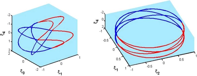

  

  Period-four orbit appears at $K=1.5$

  Figure 10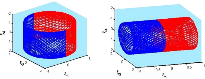

  

  Invariant torus appears at $K=1.51$

  Figure 11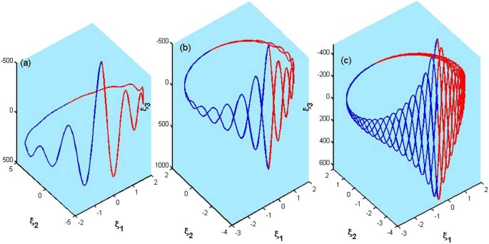

  

  Transition from period-one orbit to period-two orbit and period-five orbit due to varying of $K=24$, $K=25$, and $K=24.4$, respectively

  Figure 12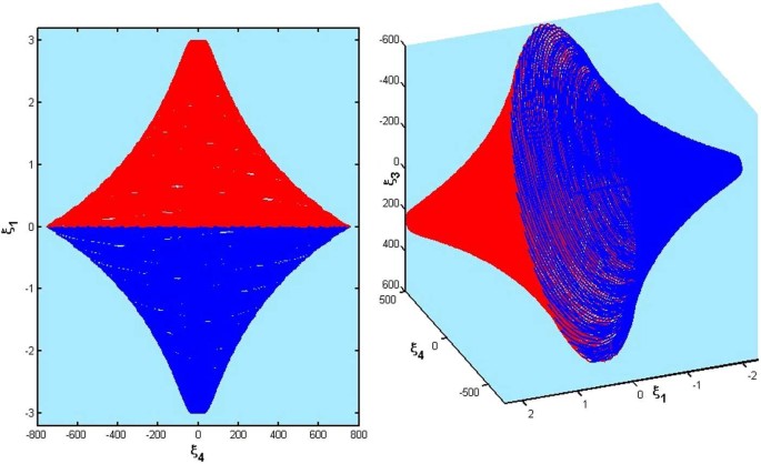

  

  Invariant torus appears at $K=24.4321$

4 Conclusion

In this paper, we have discussed the bifurcation of period-$\mathcal{K}$ orbit of a class of four-dimensional homogeneous linear SDSs in two possible behaviors: transversal crossing and attractive sliding mode. Using the generalized iterate of a Poincaré map, we have seen that in the transition from period-one orbit into period-two orbit, the system has at least three families of invariant cones. These phenomena cannot be predicted for certain three-dimensional homogeneous linear SDSs. Moreover, we have proved the existence in this system of several types of bifurcation boundaries such as multi-sliding bifurcation, invariant torus, crossing-sliding, and grazing-sliding.

In the forthcoming work, we will consider the situation that the boundaries of the sliding region intersect transversally, where $\xi\in \mathcal {M}^{0}$ is a two-fold singularity (see Lemma 1 and Fig. 2). This can have a dramatic effect, and we will give a classification of the existence of invariant cones nearby.

What is more, the future direction of this work includes the studies of discontinuous fractional-order systems due to the unique nature of these systems and effect of fractional parameter. On the other hand, these systems are usually used to model various problems in biological and engineering research. For instance, it was shown that the fractional-order systems occur as models in many applications, see [1, 2, 11, 20, 24]. The mathematical formulation of these examples leads naturally to theoretical and numerical analysis of fractional-order systems. Therefore, we will begin to develop a numerical method for integrating discontinuous fractional-order systems. This method is based on the integration of non-smooth parts and piecing these parts together with appropriate transition conditions, also taking into account that phenomena of bifurcations between these parts can also occur.

References

Alipour, M., Arshad, S., Baleanu, D.: Numerical and bifurcations analysis for multi-order fractional model of HIV infection of CD4 T-cells. UPB Sci. Bull., Ser. A 78(4), 243–258 (2016)
Babakhani, A., Baleanu, D., Khanbabaie, R.: Hopf bifurcation for a class of fractional differential equations with delay. Nonlinear Dyn. 69(3), 101–116 (2012)
Brogliato, B.: Nonsmooth Mechanics – Models, Dynamics and Control. Springer, London (1999)
Carmona, V., Fernández-García, S., Freire, E.: Saddle-node bifurcation of invariant cones in 3d piecewise linear systems. Phys. D: Nonlinear Phenom. 241, 623–635 (2012)
di Bernardo, M., Budd, C., Champneys, A.R., Kowalczyk, P.: Piecewise-Smooth Dynamical Systems: Theory and Applications. Applied Mathematics Series, vol. 163. Springer, London (2008)
di Bernardo, M., Budd, C., Champneys, A.R., Kowalczyk, P., Nordmark, A.B., Olivar, G., Piiroinen, P.T.: Bifurcations in nonsmooth dynamical systems. SIAM Rev. 50(4), 629–701 (2008)
Fečkan, M., Pospísil, M.: Poincaré–Andronov–Melnikov Analysis for Non-smooth Systems. Academic Press is an imprint of Elsevier, London (2016)
Golmankhaneh, A.K., Arefi, R., Baleanu, D.: The proposed modified Liu system with fractional order. Adv. Math. Phys. 2013, Article ID 186037 (2013)
Golmankhaneh, A.K., Arefi, R., Baleanu, D.: Synchronization in a nonidentical fractional order of a proposed modified system. J. Vib. Control 21(6), 1154–1161 (2015)
Hidde, D.J.: Modeling and simulation of genetic regulatory systems: a literature review. J. Comput. Biol. 9, 67–103 (2002)
Hajipour, M., Jajarmi, A., Baleanu, D.: An efficient non-standard finite difference scheme for a class of fractional chaotic systems. J. Comput. Nonlinear Dyn. 13(2), 021013 (2017)
Hosham, H.A.: Bifurcation of periodic orbits in discontinuous systems. Nonlinear Dyn. 87(1), 135–148 (2017)
Huan, S.M.: Existence and stability of invariant cones in 3-dim homogeneous piecewise linear systems with two zones. Int. J. Bifurc. Chaos 27(1), 1750007 (2017)
Huan, S.M., Yang, X.S.: Existence of chaotic invariant set in a class of 4-dimensional piecewise linear dynamical systems. Int. J. Bifurc. Chaos 24(12), 1450158 (2014)
Küpper, T.: Invariant cones for non-smooth systems. Math. Comput. Simul. 79, 1396–1409 (2008)
Küpper, T., Hosham, H.A.: Reduction to invariant cones for non-smooth systems. Math. Comput. Simul. 81, 980–995 (2011)
Küpper, T., Hosham, H.A., Dudtschenko, K.: The dynamics of bells as impacting system. J. Mech. Eng. Sci. 225(10), 2436–2443 (2011)
Küpper, T., Hosham, H.A., Weiss, D.: Bifurcation for nonsmooth dynamical systems via reduction methods. In: Johann, A., Kruse, H.-P., Rupp, F., Schmitz, S. (eds.) Recent Trends in Dynamical Systems. Proceedings in Mathematics and Statistics, vol. 35, pp. 79–105. Springer, Basel (2013)
Llibre, J., Teixeira, M.A.: Piecewise linear differential systems without equilibria produce limit cycles? Nonlinear Dyn. 88(1), 157–164 (2017)
Li, L., Wang, Z., Li, Y., Lu, J., Shen, H.: Hopf bifurcation analysis of a complex-valued neural network model with discrete and distributed delays. Appl. Math. Comput. 330, 152–169 (2018)
Makarenkov, O., Lamb, J.S.W.: Dynamics and bifurcations of nonsmooth systems: a survey. Phys. D: Nonlinear Phenom. 241, 1826–1844 (2012)
Shaw, S.W., Holmes, P.J.: A periodically forced piecewise linear oscillator. J. Sound Vib. 90, 129–155 (1983)
Thieme, H.R.: Mathematics in Population Biology. Princeton University Press, Princeton (2003)
Wang, Z., Wang, X., Li, Y., Huang, X.: Stability and Hopf bifurcation of fractional-order complex-valued single neuron model with time delay. Int. J. Bifurc. Chaos 27(13), 1750209 (2017)
Weiss, D., Küpper, T., Hosham, H.A.: Invariant manifolds for nonsmooth systems. Phys. D: Nonlinear Phenom. 241(22), 1895–1902 (2012)
Weiss, D., Küpper, T., Hosham, H.A.: Invariant manifolds for nonsmooth systems with sliding mode. Math. Comput. Simul. 110, 15–32 (2015)
Wu, T., Yang, X.S.: Construction of a class of four-dimensional piecewise affine systems with homoclinic orbits. Int. J. Bifurc. Chaos 26(6), 1650099 (2016)
Acknowledgements
The author is thankful to the reviewers for their useful corrections and suggestions, which improved the quality of this paper.
Availability of data and materials
Not applicable.
Funding
Not applicable. (No funding was received.)
Author information
Authors and Affiliations
Contributions
The author read and approved the final manuscript.
Corresponding author
Ethics declarations
Competing interests
I declare that I have no significant competing financial, professional, or personal interests that might have influenced the performance or presentation of the work described in this manuscript.
Additional information
Publisher’s Note
Springer Nature remains neutral with regard to jurisdictional claims in published maps and institutional affiliations.
Rights and permissions
Open Access This article is distributed under the terms of the Creative Commons Attribution 4.0 International License (http://creativecommons.org/licenses/by/4.0/), which permits unrestricted use, distribution, and reproduction in any medium, provided you give appropriate credit to the original author(s) and the source, provide a link to the Creative Commons license, and indicate if changes were made.
About this article
Cite this article
Hosham, H.A. Bifurcations in four-dimensional switched systems. Adv Differ Equ 2018, 388 (2018). https://doi.org/10.1186/s13662-018-1850-1
Received:
Accepted:
Published:
DOI: https://doi.org/10.1186/s13662-018-1850-1