Modulational instability and higher-order rogue wave solutions for an integrable generalization of the nonlinear Schrödinger equation in monomode optical fibers

Abstract

We consider the integrable generalization of the nonlinear Schrödinger equation that arises as a model for nonlinear pulse propagation in monomode optical fibers. The existent conditions for its modulational instability to form the rogue waves is given from its plane-wave solutions. We propose a generalized $(n,N-n)$-fold Darboux transformation for this system by using the Nth-order Darboux matrix, Taylor expansion, and a limit procedure. As an application, we use the generalized perturbation $(1,N-1)$-fold Darboux transformation to generate higher-order rogue wave solutions of this system. The dynamics behavior of the first-, second-, and third-order rouge wave solutions are shown graphically. These results may be useful for understanding some physical phenomena in optical fibers.

1 Introduction

Recently, rogue waves (RWs) have attracted more and more theoretical and experimental attention [1]. The RWs were first observed in deep oceans, and later these studies gradually extended to other fields, such as fiber optics, Bose-Einstein condensates, and capillary waves [2–5]. In fact, RWs are taken as a new type of explicit rational solutions of nonlinear wave equations. The nonlinear Schrödinger equation is one of the most fundamental modes admitting RWs [2]. Until now, many nonlinear Schrödinger-type equations have been reported to have rogue wave solutions [6–11]. In [6], multirogue wave solutions of a Schrödinger equation with higher-order terms employing the generalized DT and some related properties of the nonautonomous rogue waves are investigated analytically. Based on the similarity transformation, several families of nonautonomous wave solutions have been studied for the generalized coupled cubic-quintic nonlinear Schrödinger equation with group-velocity dispersion, fiber gain-or-loss, and nonlinearity coefficient functions, which describes the evolution of a slowly varying wave packet envelope in the inhomogeneous optical fiber [7]. The Nth-order rogue wave solutions have been obtained for a higher-order variable coefficients nonlinear Schrödinger equation, which plays an important role in the control of the ultrashort optical pulse propagation in nonlinear optical systems [8]. Based on the Nth-iterated generalized DT formula, the vector bright soliton solution and vector rogue wave solution have been systematically derived for the coherently coupled nonlinear Schrödinger system [9]. In [10, 11], the authors have presented some soliton, breather, and rogue wave solutions for the $(2+1)$-dimensional derivative nonlinear Schrödinger equation and $(2+1)$-dimensional nonlinear Schrödinger equation via the Nth-order generalized Darboux transformation. In the present paper, based on our proposed generalized $(n,N-n)$-fold DT method by using the Taylor expansion of the Darboux matrix [4, 5], which is different from the iterated generalized DT in [2, 3, 6–11], we will investigate the following integrable generalization of the nonlinear Schrödinger equation (gNLS) [12–14]:

$$ u_{xt}+\alpha\beta^{2} u -2i \alpha\beta u_{x}- \alpha u_{xx}-i\alpha \beta^{2} |u|^{2}u_{x} =0, $$

(1)

where $u= u(x,t)$ is the slowly varying complex envelope of the wave, α and β are real constants, and i is the imaginary number unit ($i^{2}=-1$). Equation (1) may model nonlinear pulse propagation in monomode optical fibers. In [12], an N-fold DT is constructed for Eq. (1), one- and two-soliton solutions are obtained from the trivial solution, and two classes of new explicit solutions are given explicitly from a plane wave solution as the seeding solution. For some relevant research results on Eq. (1), we refer the reader to [12–14] and references therein. However, Eq. (1) is different from other NLS equation and its generalization forms [2, 3, 6–11, 15–18] owing to the term $u_{xt}$; to the best of our knowledge, the modulational instability, generalized $(n,N-n)$-fold DT, and higher-order rogue wave solutions for Eq. (1) have not been studied yet.

So, in this paper, we make further investigation on Eq. (1) via our proposed generalized $(n,N-n)$-fold DT technique [4, 5]. The rest of the paper is as follows. In Section 2, the modulational instability of Eq. (1) is investigated. In Section 3, based on the DT in [12], we give a brief introduction to the N-fold DT of Eq. (1). In Section 4, we construct the generalized $(n,N-n)$-fold DT of Eq. (1). In Section 5, based on the generalized $(1,N-1)$-fold DT, we give some higher-order rogue wave solutions, and the dynamics behavior of those solutions are shown by some figures. Finally, we address the conclusions in Section 6.

2 Modulational instability of plane wave states

Before we study higher-order RW solutions of Eq. (1), we investigate the modulational instability of Eq. (1). We start with its plane wave solution in the form

$$ u=ce^{i[ax+(\alpha a+2\alpha\beta+\alpha\beta^{2} c^{2}+\frac{\alpha\beta ^{2}}{a})t]}, $$

(2)

where c is a real amplitude, and a is a real wave number. Substituting the perturbation solution $u(x,t)=[c+\varepsilon U(x,t)]e^{i[ax+(\alpha a+2\alpha\beta+\alpha\beta^{2} c^{2}+\frac{\alpha\beta^{2}}{a})t]}$ into Eq. (1) yields the linearized equation (only considering the linear term of ε)

$$ U_{x,t}+\alpha\beta^{2} U+ i U_{t}+i \alpha \beta^{2} U_{x}-i \alpha U_{x}+\alpha \beta^{2} U^{*}_{x}-\alpha U_{xx}=0. $$

(3)

We consider the solution to Eq. (3) with the wave number k and frequency ω in the form

$$ U=F \cos(k x-\omega t)+i G \sin(k x-\omega t), $$

(4)

where F and G are real amplitudes. Substituting (4) into (3) yields the following dispersion relation for the perturbations, obtained as the condition for the existence of nontrivial solutions for F and G (i.e., $FG\neq0$):

$$ \omega=\frac{\alpha k(a k^{2}-a^{3}+a^{2}\beta^{2} c^{2}+a\beta ^{2}\pm\beta^{2}\sqrt{a^{4} c^{4}+2 a^{3} c^{2}+k^{2}})}{a(a^{2}-k^{2})}. $$

(5)

When $a^{4} c^{4}+2 a^{3} c^{2}+k^{2}<0$, the frequency ω becomes complex, and the disturbance grows with time exponentially. In the following, we consider the gain spectrum of modulational instability. The power gain is obtained from (5) by

$$ g(k)=\operatorname{Im}(\omega)=\frac{|\alpha k \beta^{2}|\sqrt{-a^{4} c^{4}-2 a^{3} c^{2}-k^{2}}}{|a(a^{2}-k^{2})|},$$

(6)

where $g(k)$ stands for the gain with $a^{4} c^{4}+2 a^{3} c^{2}+k^{2}<0$. In what follows, we assume that $\alpha=\beta=1$ and $a=-\frac{1}{c^{2}}$ and choose different values of the parameter c, showing the gain spectra at five power levels in Figure 1.

Figure 1

Gain spectra of modulation instability for the different parameter values $\pmb{c = 0.5; 0.75; 1; 1.5; 2}$ . (Color online.)

3 The N-fold DT for Eq. (1)

In this part, we give a brief introduction of the N-fold DT for Eq. (1). According to [12], the Lax pair for Eq. (1) is as follows:

$$\begin{aligned}& \varphi_{x}=U \varphi_{n} = \left ( \textstyle\begin{array}{@{}c@{\quad}c@{}} - i\frac{1}{\lambda^{2}} & \frac{u_{x}}{\lambda} \\ - \frac{u^{*}_{x}}{\lambda} & i\frac{1}{\lambda^{2}} \end{array}\displaystyle \right ) \varphi, \end{aligned}$$

(7)

$$\begin{aligned}& \varphi_{t}=V \varphi_{n} = \left ( \textstyle\begin{array}{@{}c@{\quad}c@{}} \frac{i}{2} \alpha\beta^{2}|u|^{2}-i\mu^{2} & \frac{\alpha}{\lambda }u_{x}+\frac{i}{2} \alpha\beta^{2}u \\ -\frac{\alpha}{\lambda}{u^{*}}_{x}+\frac{i}{2} \alpha\beta^{2} u^{*} & -\frac{i}{2} \alpha\beta^{2}|u|^{2}+i\mu^{2} \end{array}\displaystyle \right ) \varphi, \end{aligned}$$

(8)

where ∗ represents the complex conjugation, $\varphi=(\phi,\psi)^{\mathrm{T}}$ (the superscript T denotes the vector transpose) is the vector eigenfunction, λ is the spectral parameter, and $\mu=\sqrt {\alpha}(\frac{1}{\lambda}-\frac{1}{2}\beta\lambda)$. Here, to construct RW solutions for Eq. (1), it is worth pointing out that we have changed the spectral parameter of Lax pair from λ to $\frac{1}{\lambda}$ in [12]. The compatibility condition $U_{t}-V_{x}+UV-VU=0$ between Eqs. (7) and (8) gives rise to Eq. (1). In the following, we proceed by establishing the N-fold DT of Eq. (1). For this reason, we introduce the transformation

$$ \tilde{\varphi}=T \varphi, $$

(9)

where φ̃ is required to satisfy Eqs. (7) and (8) with U and V replaced by Ũ and Ṽ, that is,

$$\begin{aligned}& \tilde{\varphi}=\widetilde{U} \tilde{\varphi}, \qquad \widetilde {U}=(T_{t}+T U) {T}^{-1}, \end{aligned}$$

(10)

$$\begin{aligned}& \tilde{\varphi}_{t}=\widetilde{V} \tilde{\varphi},\qquad \widetilde {V}=(T_{t}+T V) {T}^{-1}. \end{aligned}$$

(11)

Hereby, we assume that theNth-order Darboux matrix T is of the form

$$ T = \left ( \textstyle\begin{array}{@{}c@{\quad}c@{}} A & B\\ C & D \end{array}\displaystyle \right )= \left ( \textstyle\begin{array}{@{}c@{\quad}c@{}} \lambda^{2N}+\sum_{j=0}^{N-1}A^{(2j)}\lambda^{2j} &\sum_{j=0}^{N-1}B^{(2j+1)} \lambda^{2j+1} \\ -\sum_{j=0}^{N-1}{B^{(2j+1)}}^{*} \lambda^{2j+1} &\lambda^{2N}+\sum_{j=0}^{N-1}{A^{(2j)}}^{*}\lambda^{2j} \end{array}\displaystyle \right ) $$

(12)

with the complex functions $A^{(2j)}$ and $B^{(2j+1)}$ ($j=0,1,2,\ldots ,N-1$) solving the linear system $T(\lambda_{k})\varphi(\lambda_{k})=0$ ($k=1,2,\ldots,N$), that is,

$$ \begin{aligned} &\Biggl(\lambda^{2N}+\sum _{j=0}^{N-1}A^{(2j)}\lambda^{2j} \Biggr)\phi+\Biggl(\sum_{j=0}^{N-1}B^{(2j+1)} \lambda^{2j+1}\Biggr) \psi=0, \\ &\Biggl(-\sum_{j=0}^{N-1}{B^{(2j+1)}}^{*} \lambda^{2j+1}\Biggr)\phi+\Biggl(\lambda ^{2N}+\sum _{j=0}^{N-1}{A^{(2j)}}^{*} \lambda^{2j}\Biggr) \psi=0, \end{aligned} $$

(13)

where $\varphi(\lambda_{k})=(\phi(\lambda_{k}), \psi(\lambda_{k}))^{\mathrm{T}}=(\phi_{k}, \psi_{k})$ is a basic solution of Eqs. (7) and (8) for the given spectral parameter $\lambda_{k}$ and seed solution $u_{0}$. Of course, it should be noted that the Darboux matrix (12) here is a little different from that in [12], owing to the variation of the spectral parameter λ in Lax pair. The 2N nonzero variables $A^{(2j)}$ and $B^{(2j+1)}$ can be determined by 2N equations in (13) when the spectral parameters $\lambda_{k}$ are suitably chosen.

According to the steps in [12], the usual N-fold Darboux transformation of Eq. (1) is given by

$$ \tilde{u}_{N-1}=u+ {B^{(2N-1)}}, $$

(14)

where $B^{(2N-1)}(x,t)=\frac{\Delta B^{(2N-1)}}{\Delta_{N}}$ with

$$\Delta_{N} = \left \vert \textstyle\begin{array}{@{}c@{\quad}c@{\quad}c@{\quad}c@{\quad}c@{\quad}c@{\quad}c@{\quad}c@{}} \lambda_{1}^{2(N-1)}\phi_{1} & {\lambda_{1}}^{2(N-2)}\phi_{1} &\cdots & \phi_{1} & {\lambda_{1}}^{2N-1}\psi_{1} & \lambda_{1}^{2N-3}\psi_{1} &\cdots& \lambda _{1}\psi_{1} \\ \lambda_{2}^{2(N-1)}\phi_{2} & {\lambda_{2}}^{2(N-2)}\phi_{2} &\cdots & \phi_{2} & {\lambda_{2}}^{2N-1}\psi_{2} & \lambda_{2}^{2N-3}\psi_{2} &\cdots& \lambda _{2}\psi_{2} \\ \cdots& \cdots &\cdots &\cdots&\cdots& \cdots &\cdots &\cdots \\ \lambda_{N}^{2(N-1)}\phi_{N} & {\lambda_{N}}^{2(N-2)}\phi_{N} &\cdots & \phi_{N} & {\lambda_{N}}^{2N-1}\psi_{N} & \lambda_{N}^{2N-3}\psi_{N} &\cdots& \lambda _{N}\psi_{N} \\ \lambda_{1}^{*2(N-1)}\psi^{*}_{1} & {\lambda_{1}}^{*2(N-2)}\psi_{1}^{*} &\cdots & \psi_{1}^{*} & -\lambda_{1}^{*(2N-1)}\phi_{1} & -\lambda _{1}^{*(2N-3)}\phi_{1}^{*} &\cdots& -\lambda_{1}^{*}\phi_{1}^{*} \\ \lambda_{2}^{*2(N-1)}\psi^{*}_{2} & {\lambda_{2}}^{*2(N-2)}\psi_{2}^{*} &\cdots & \psi_{2}^{*} & -\lambda_{2}^{*(2N-1)}\phi_{2} & -\lambda _{2}^{*(2N-3)}\phi_{2}^{*} &\cdots& -\lambda_{2}^{*}\phi_{2}^{*} \\ \cdots& \cdots &\cdots &\cdots&\cdots& \cdots &\cdots &\cdots \\ \lambda_{N}^{*2(N-1)}\psi^{*}_{N} & {\lambda_{N}}^{*2(N-2)}\psi_{N}^{*} &\cdots & \psi_{N}^{*} & -\lambda_{N}^{*(2N-1)}\phi_{N} & -\lambda _{N}^{*(2N-3)}\phi_{N}^{*} &\cdots& -\lambda_{N}^{*}\phi_{N}^{*} \end{array}\displaystyle \right \vert , $$

and $\Delta B^{(2N-1)}$ is given by the determinant $\Delta_{N}$ by replacing its $(N+1)$th column by the column vector $(-\lambda _{1}^{2N}\phi_{1}, -\lambda_{2}^{2N}\phi_{2},\ldots, -\lambda_{N}^{2N}\phi _{N}, -\lambda_{1}^{*(2N)}\psi_{1}^{*}, -\lambda_{2}^{*(2N)}\psi _{2}^{*},\ldots, -\lambda_{N}^{*(2N)}\psi_{N}^{*})^{\mathrm{T}}$.

For the proof of the form invariance for Ũ, Ṽ and U, V, we refer to [12, 19, 20] and references therein, where the proof process is similar. The aim of this paper is to construct the generalized $(n,N-n)$-fold DT and higher-order rogue wave solutions in terms of determinants. Hereby, the proof is omitted for simplicity. Transformations (9) and (14) are called an N-DT of Eq. (1). By applying the N-fold DT, higher-order soliton solutions (or higher-order breather solutions) for Eq. (1) are obtained by choosing the constant seed solution (or plane wave solutions) [12].

4 Generalized $(n,N-n)$-fold DT for Eq. (1)

For the N-fold DT with N distinct spectral parameters, we can derive a 2N-soliton solution in terms of the determinant representation. However, for the generalized $(n,N-n)$-fold DT for Eq. (1), the main difference is that we can adjust the number of the spectral parameter: the least may be 1, and the most may be N. Here, we consider the case with n distinct spectral parameters $\lambda_{i}$ ($i=1,2,\ldots,n$), $1\leq n\leq N$.

Here we still consider the Darboux matrix (12), but with n spectral parameters $\lambda_{i}$ ($i=1,2,\ldots,n$), $1\leq n\leq N$, and not with N ($N>1$) distinct spectral parameters, in which the condition $T(\lambda_{i})\varphi(\lambda_{i})=0$ leads to the linear algebraic system with only 2n equations

$$ \begin{aligned} & \Biggl[\lambda_{i}^{2N}+\sum _{j=0}^{N-1}A^{(2j)} \lambda_{i}^{2j} \Biggr]\phi (\lambda_{i}) +\sum _{j=0}^{N-1}B^{(2j+1)} \lambda^{2j+1}_{1}\psi(\lambda_{i})=0, \\ & \Biggl[\lambda_{i}^{*(2N)}+\sum _{j=0}^{N-1}{A^{(2j)}}\lambda _{i}^{*(2j)} \Biggr]\psi^{*}(\lambda_{i})- \sum_{j=0}^{N-1}{B^{(2j+1)}} \lambda_{i}^{*(2j+1)}\phi^{*}(\lambda_{i})=0, \end{aligned} $$

(15)

where $\varphi(\lambda_{i})=(\phi(\lambda_{i}), \psi(\lambda_{i}))^{\mathrm {T}}$ is a solution of the linear spectral problem (7) and (8) with one spectral parameter $\lambda=\lambda_{i}$ and the initial solution $u_{0}$ of Eq. (1). When $n< N$, we only have 2n above-given algebraic constraints (15) for 2N unknown functions $A^{(2j)}$ and $B^{(2j+1)}$ ($j=0,1,\ldots,N-1$). This means that the number of the unknown variables $A^{(2j)}$ and $B^{(2j+1)}$ is greater than that of equations, so that we have some free functions. To determine these 2N unknown functions $A^{(2j)}$ and $B^{(2j+1)}$, we need to find additional $2(N-n)$ equations for 2N functions $A^{(2j)}$ and $B^{(2j+1)}$ so that we would have 2N equations for 2N functions $A^{(2j)}$ and $B^{(2j+1)}$. Determining these 2N functions $A^{(2j)}$ and $B^{(2j+1)}$, we then can obtain ‘new’ solutions of Eq. (1) in terms of DT.

To generate ‘new’ additional $2(N-n)$ equations from $T(\lambda _{i})\varphi(\lambda_{i})=0$, we consider the Taylor expansion of $T(\lambda _{i}+\varepsilon)\varphi(\lambda_{i}+\varepsilon)$ ($i=1,2,\ldots,n$) at $\varepsilon=0$. We know that

$$ \varphi(\lambda_{i}+\varepsilon)=\varphi^{(0)}( \lambda_{i})+\varphi ^{(1)}(\lambda_{i})\varepsilon +\varphi^{(2)}(\lambda_{i})\varepsilon^{2}+\cdots, $$

(16)

where $\varphi^{(k)}(\lambda_{i})=\frac{1}{k!}\frac{\partial^{k}}{\partial \lambda_{i}^{k}}\varphi(\lambda_{i})= (\frac{1}{k!}\frac{\partial ^{k}}{\partial\lambda_{i}^{k}}\phi(\lambda_{i}), \frac{1}{k!}\frac{\partial ^{k}}{\partial\lambda_{i}^{k}}\psi(\lambda_{i}) )^{\mathrm{T}}$ with $\varphi^{(0)}(\lambda_{i})=\varphi(\lambda_{i})=(\phi(\lambda_{i}), \psi (\lambda_{i}))^{\mathrm{T}}$ ($k=0,1,2,\ldots$), and

$$ T(\lambda_{i}+\varepsilon)=T(\lambda_{i})+\sum _{k=1}^{2N} T^{(k)}(\lambda _{i}) \varepsilon^{k}. $$

(17)

Thus, we have

$$ T(\lambda_{i}+\varepsilon) \varphi(\lambda_{i}+ \varepsilon) =\sum_{k=0}^{+\infty}\sum _{j=0}^{k}T^{(j)}(\lambda_{1}) \varphi ^{(k-j)}(\lambda_{i})\varepsilon^{k}, $$

(18)

where $\varphi_{i}^{(k)}(\lambda_{i})=\frac{1}{k!}\frac{\partial ^{k}}{\partial\lambda_{i}^{k}}\varphi_{i}(\lambda)|_{\lambda=\lambda_{i}}$, and ε is a small parameter.

It follows from Eq. (18) and

$$ \lim_{\varepsilon\to0}\frac{T(\lambda_{i}+\varepsilon) \varphi(\lambda _{i}+\varepsilon)}{\varepsilon^{k_{i}}}=0 $$

(19)

for $i=1,2,\ldots,n$ and $k_{i}=0,1,\ldots,m_{i}$ that we obtain the linear algebraic system with 2N equations ($N=n+\sum_{i=1}^{n}m_{i}$, $i=1,2,\ldots,n$):

$$ \begin{aligned} &T^{(0)}(\lambda_{i}) \varphi^{(0)}(\lambda_{i})=0, \\ &T^{(0)}(\lambda_{i})\varphi^{(1)}( \lambda_{i})+T^{(1)}(\lambda_{i})\varphi ^{(0)}(\lambda_{i})=0, \\ &\ldots, \\ &\sum_{j=0}^{m_{i}}T^{(j)}( \lambda_{i})\varphi^{(m_{i}-j)}(\lambda_{i})=0, \end{aligned} $$

(20)

in which we have some first systems for every index i, that is, $T^{(0)}(\lambda_{i})\varphi^{(0)}(\lambda_{i})=T(\lambda_{i})\varphi(\lambda _{i})=0$ are just ones in system (13), but they are different if there exist at least one index $m_{i}\neq0$. Here the number $m_{i}$ ($m_{i}=0,1,2,\ldots$) is the highest order perturbation derivatives corresponding to $\lambda_{i}$ ($i=1,2,\ldots,n$), where the nonnegative integers n, $m_{i}$ are required to satisfy $N=n+\sum_{i=1}^{n}m_{i}$, and N is the same as in the Darboux matrix T (12).

Therefore, we have obtained system (20) containing 2N algebraic equations with 2N unknowns functions $A^{(2j)}$ and $B^{(2j+1)}$ ($j=0,1,\ldots,N-1$). When the eigenvalue $\lambda_{i}$ is suitably chosen so that the determinant of the coefficients for system (20) is nonzero, the transformation matrix T is uniquely determined by system (20). It can be shown that the above N-fold DT still holds for the Darboux matrix (12) with $A^{(2j)}$, $B^{(2j+1)}$ ($j=0,1,\ldots,N-1$) determined by system (20). Owing to new distinct functions $A^{(2j)}$, $B^{(2j+1)}$ obtained in the Nth-order Darboux matrix T, we can derive the ‘new’ DT with the n eigenvalues $\lambda=\lambda_{i}$. We call Eqs. (9) and (14) associated with new functions $A^{(2j)}$, $B^{(2j+1)}$ determined by system (20) a generalized $(n,N-n)$-fold DT. So we have the following theorem for the generalized $(n,N-n)$-fold DT of Eq. (1).

Theorem 1

The spectral problem (7)-(8) is covariant with respect to the transformations (9), and

$$ \tilde{u}_{N}=u+ {B^{(2N-1)}}, $$

(21)

with $B^{(2N-1)}=\frac{\Delta^{\epsilon(n)}B^{(2N-1)}}{\Delta _{N}^{\epsilon(n)}}$ defined by solving the linear algebraic system (20) in terms of the Cramer rule, where $\Delta_{N}^{\epsilon (n)}=\operatorname{det}([\Delta^{(1)}\cdots\Delta^{(n)}]^{\mathrm{T}})$ with

$$\begin{aligned} \begin{aligned}[b] &\Delta^{(i)} \\ &\quad = \left [ \textstyle\begin{array}{@{}c@{\quad}c@{\quad}c@{\quad}c@{\quad}c@{\quad}c@{\quad}c@{\quad}c@{}} {\lambda_{i}}^{2N-2} {\phi_{i}^{(0)}} & {\lambda_{i}}^{2N-4} {\phi_{i}^{(0)}} &\cdots& {\phi_{i}^{(0)}} & {\lambda_{i}}^{2N-1} {\psi_{i}^{(0)}} & {\lambda _{i}}^{2N-3} {\psi_{i}^{(0)}} &\cdots& \lambda_{i}\psi_{i}^{(0)} \\ \Delta_{2,1}^{(i)}& \Delta_{2,2}^{(i)} &\cdots&{\phi_{i}^{(1)}} & \Delta _{2,N+1}^{(i)} & \Delta_{2,N+2}^{(i)} &\cdots& \Delta_{2,2N}^{(i)} \\ \vdots& \vdots &\ddots &\vdots&\vdots& \vdots &\ddots &\vdots \\ \Delta_{m_{i}+1,1}^{(i)} & \Delta_{m_{i}+1,2}^{(i)} &\cdots&{\phi _{i}^{(m_{i})}} &\Delta_{m_{i}+1,N+1}^{(i)} & \Delta_{m_{i}+1,N+2}^{(i)} &\cdots& \Delta_{m_{i}+1,2N}^{(i)} \\ {\lambda_{i}^{*}}^{(2N-2)} {\psi_{i}^{(0)}}^{*} & {\lambda_{i}^{*}}^{(2N-4)} {\psi _{i}^{(0)}}^{*} &\cdots& {\psi_{i}^{(0)}}^{*} & -{\lambda_{i}^{*}}^{(2N-1)} {\phi _{i}^{(0)}}^{*} & -{\lambda_{i}^{*}}^{(2N-3)} {\phi_{i}^{(0)}}^{*} &\cdots& -\lambda_{i}^{*}{\phi_{i}^{(0)}}^{*} \\ \Delta_{m_{i}+3,1}^{(i)} & \Delta_{m_{i}+3,2}^{(i)} &\cdots&{\psi _{i}^{(1)}}^{*} &\Delta_{m_{i}+3,N+1}^{(i)} & \Delta_{m_{i}+3,N+2}^{(i)} &\cdots& \Delta_{m_{i}+3,2N}^{(i)} \\ \vdots& \vdots &\ddots &\vdots&\vdots& \vdots &\ddots &\vdots \\ \Delta_{2(m_{i}+1),1}^{(i)} & \Delta_{2(m_{i}+1),2}^{(i)} &\cdots&{\psi _{i}^{(m_{i})}}^{*} &\Delta_{2(m_{i}+1),N+1}^{(i)} & \Delta _{2(m_{i}+1),N+2}^{(i)} &\cdots&\Delta_{2(m_{i}+1),2N}^{(i)} \end{array}\displaystyle \right ] \end{aligned} \end{aligned}$$

(22)

and $\Delta_{j,s}^{(i)}$ ($1\leq j\leq2(m_{i}+1)$, $1\leq s\leq N$ $i=1,2,\ldots,n$) given by the following formulae:

$$ \Delta_{j,s}^{(i)}= \textstyle\begin{cases} \sum_{k=0}^{j-1}C^{k}_{2N-2s} {\lambda_{i}}^{2N-2s-k} {\phi_{i}^{(j-1-k)}}& \textit{for } 1\leq j\leq m_{i}+1, \\ &\hphantom{\textit{for }}1\leq s\leq N, \\ \sum_{k=0}^{j-1}C^{k}_{4N-2s+1} {\lambda_{i}}^{4N-2s+1-k} {\psi _{i}^{(j-1-k)}}& \textit{for } 1\leq j\leq m_{i}+1, \\ &\hphantom{\textit{for }} N+1\leq s\leq2N, \\ \sum_{k=0}^{j-(N+1)}C^{k}_{2N-2s} {\lambda_{i}}^{*(2N-2s-k)} {\psi _{i}^{(j-N-1-k)*}}& \textit{for } m_{i}+2\leq j\leq2(m_{i}+1), \\ &\hphantom{\textit{for }} 1\leq s\leq N, \\ -\sum_{k=0}^{j-(N+1)}C^{k}_{4N-2s+1} {\lambda_{i}}^{*(4N-2s+1-k)} {\phi _{i}^{(j-N-1-k)*}}& \textit{for } m_{i}+2\leq j\leq2(m_{i}+1), \\ &\hphantom{\textit{for }} N+1\leq s\leq2N, \end{cases} $$

(23)

and $\Delta^{\epsilon} {B^{(2N-1)}}$ is formed from the determinant $\Delta_{N}^{\epsilon(n)}$ by replacing its $(N+1)$ th column by the column vector $(b^{(1)}\cdots b^{(n)})^{\mathrm {T}}$ with $b^{(i)}=(b_{j}^{(i)})_{2(m_{i}+1)\times1}$ and

$$ b_{j}^{(i)}= \textstyle\begin{cases} -\sum_{k=0}^{j-1}C^{k}_{2N} {\lambda_{i}}^{2N-k} {\phi_{i}^{(j-1-k)}}& \textit {for } 1\leq j\leq m_{i}+1, \\ -\sum_{k=0}^{j-(N+1)}C^{k}_{2N} {\lambda _{i}}^{*(2N-k)} {\psi_{i}^{(j-N-1-k)*}}& \textit{for } m_{i}+2\leq j\leq2(m_{i}+1). \end{cases} $$

(24)

Notice that when $n=N$ (i.e., $m_{i}=0$, $1\leq i\leq N$), Theorem 1 reduces to the N-fold DT; when $n=1$ and $m_{1}=N-1$, Theorem 1 reduces to the $(1,N-1)$-fold DT. Here, we remark that system (20) in the generalized $(n,N-n)$-fold DT is very important; its role is similar to that of Eqs. (13) of the N-fold DT; both of them can determine the 2N unknown functions $A^{(2j)}$, $B^{(2j+1)}$ ($0\leq j\leq N-1$), but they are different from each other: Eqs. (13) have 2N spectral parameters, whereas system (20) only has 2n spectral parameters. Owing to different $A^{(2j)}$, $B^{(2j+1)}$ ($0\leq j\leq N-1$), the former can lead to the N-soliton solutions, whereas the latter may generate higher-order rogue wave solutions. In the following, we will use the generalized perturbation $(1, N-1)$-fold Darboux transformation to investigate higher-order rogue wave solutions of the gNLS equation (1) from the initial plane wave solution.

5 Higher-order RWs of Eq. (1)

In this section, we give some rogue wave solutions in terms of determinants of Eq. (1) using the generalized $(1,N-1)$-fold DT in Theorem 1 with $n=1$. Starting from the seed solution $u_{0}=ce^{i[ax+(\alpha a+2\alpha\beta+\alpha\beta^{2} c^{2}+\frac{\alpha \beta^{2}}{a})t]}$ of Eq. (1), we can give a basic solution of Lax pair (7) and (8) as follows:

$$ \varphi=\left ( \textstyle\begin{array}{@{}c@{}} (C_{1} e^{-A}+C_{2} e^{A})e^{B}\\ (-C_{1} e^{A}+C_{2} e^{-A}) e^{-B} \end{array}\displaystyle \right ) $$

(25)

with

$$\begin{aligned}& C_{1}=\sqrt{\frac{(2+\lambda^{2} a)+\sqrt{a^{2}\lambda^{4}+4+4\lambda^{2} a+4 a^{2}c^{2}\lambda^{2}}}{2a c\lambda}}, \\& C_{2}=\sqrt{ \frac{-(2+\lambda^{2} a)+\sqrt {a^{2}\lambda^{4}+4+4\lambda^{2} a+4 a^{2}c^{2}\lambda^{2}}}{2a c\lambda}}, \\& B=\frac{i}{2}\biggl[a x+\biggl(\alpha a+\alpha\beta^{2} c^{2}+2\alpha\beta+\frac{\alpha \beta^{2}}{a}\biggr)t\biggr], \\& A= \frac{i \sqrt{a^{2}\lambda^{4}+4+4\lambda^{2} a+4 a^{2}\lambda ^{2} c^{2}}(2 a x+(2 a\alpha+\alpha\beta^{2}\lambda^{2}) t+\Theta(\varepsilon ))}{4\lambda^{2} a}, \\& \Theta(\varepsilon)=\sum_{k=1}^{N}(b_{k}+d_{k} i)\varepsilon^{2k}, \end{aligned}$$

where ε is a small parameter, and $b_{k}$, $d_{k}$ ($k=1,2,\ldots,N$) are real free parameters that can control different rogue wave structures.

Next, we fix $\lambda_{1}=-\frac{\sqrt{-2a(1+a c^{2}+\sqrt{2 a c^{2}+a^{2} c^{4}})}}{a}$ and set $\lambda=\lambda_{1}+\varepsilon^{2}$ in (25). Then we expand the vector function φ in (25) as Taylor series at $\varepsilon=0$. Because the expansion expression of $\varphi (\varepsilon^{2})$ is too complicated, in the following discussions, we may set $a=-\frac{1}{c^{2}}$ to simplify our calculation process at the same time, that is, $\lambda_{1}=c(1+i)$. Therefore, we obtain

$$ \varphi\bigl(\varepsilon^{2}\bigr)=\varphi^{(0)}+\varphi ^{(1)}\varepsilon^{2}+\varphi^{(2)} \varepsilon^{4}+\varphi^{(3)}\varepsilon ^{6}+\cdots, $$

(26)

where

$$ \begin{aligned} &\varphi^{(0)}=\left ( \textstyle\begin{array}{@{}c@{}} \phi^{(0)}\\ \psi^{(0)} \end{array}\displaystyle \right ) =\left ( \textstyle\begin{array}{@{}c@{}} e^{\frac{i}{2}(-x-\alpha t+2\alpha\beta t)}\sqrt{2}\\ -i e^{-\frac{i}{2}(-x-\alpha t+2\alpha\beta t)}\sqrt{2} \end{array}\displaystyle \right ), \\ &\varphi^{(1)}=\left ( \textstyle\begin{array}{@{}c@{}} \phi^{(1)}\\ \psi^{(1)} \end{array}\displaystyle \right ), \qquad \varphi^{(2)}=\left ( \textstyle\begin{array}{@{}c@{}} \phi^{(2)}\\ \psi^{(2)} \end{array}\displaystyle \right ), \qquad \varphi^{(3)}=\left ( \textstyle\begin{array}{@{}c@{}} \phi^{(3)}\\ \psi^{(3)} \end{array}\displaystyle \right ),\qquad \ldots, \end{aligned} $$

(27)

and $\varphi^{(i)}=(\phi^{(i)},\psi^{(i)})^{\mathrm{T}}$ ($i=1,2,3$) are listed in the Appendix.

In the following, we discuss the higher-order rogue wave solutions of the four cases with $N=1, 2, 3, 4$ for Eq. (1). It is particularly worth pointing out that we only derive the trivial solution for the case $N=1$, which is omitted here. Relevant structure figures for other three cases $N=2, 3, 4$ are shown in Figures 2-4.

Figure 2

First-order rogue wave solution ( 30 ) with different parameters. (a1)-(a2) $c=1$, $\alpha=1$, $\beta=1$; (b1)-(b2) $c=4$, $\alpha=1$, $\beta=1$; (c1)-(c2) $c=1$, $\alpha=-1$, $\beta=1$; (d1)-(d2) $c=1$, $\alpha=4$, $\beta=1$; (e1)-(e2) $c=1$, $\alpha=1$, $\beta=4$. (Color online.)

(I) When $N=2$, solving the linear algebraic system (20) leads to

$$ B^{(3)}=\frac{\Delta B^{(3)}}{\Delta} $$

(28)

with

$$\Delta= \left \vert \textstyle\begin{array}{@{}c@{\quad}c@{\quad}c@{\quad}c@{}} \lambda^{2} \phi^{(0)} & \phi^{(0)} & \lambda^{3} \psi^{(0)} & \psi^{(0)}\\ \lambda^{2}\phi^{(1)}+ 2\lambda\phi^{(0)} & \phi^{(1)} & \lambda^{3}\psi ^{(1)}+ 3\lambda^{2}\psi^{(0)} & \lambda\psi^{(1)}+\psi^{(0)}\\ {\lambda^{*}}^{2} {\psi^{(0)}}^{*} & {\psi^{(0)}}^{*} &- {\lambda^{*}}^{3} {\phi ^{(0)}}^{*} & -{\lambda^{*}} {\phi^{(0)}}^{*}\\ {\lambda^{*}}^{2}{\psi^{(1)}}^{*}+ 2{\lambda^{*}} {\psi^{(0)}}^{*} & {\psi ^{(1)}}^{*} & - {\lambda^{*}}^{3}{\phi^{(1)}}^{*}- 3{\lambda^{*}}^{2}{\phi^{(0)}}^{*} & -{\lambda^{*}}{\phi^{(1)}}^{*}-{\phi^{(0)}}^{*} \end{array}\displaystyle \right \vert $$

and

$$\Delta B^{(3)}= \left \vert \textstyle\begin{array}{@{}c@{\quad}c@{\quad}c@{\quad}c@{}} \lambda^{2} \phi^{(0)} & \phi^{(0)} & -\lambda^{4} \phi^{(0)} & \psi ^{(0)}\\ \lambda^{2}\phi^{(1)}+ 2\lambda\phi^{(0)} & \phi^{(1)} & -\lambda^{4}\phi ^{(1)}-4\lambda^{3}\phi^{(0)} & \lambda\psi^{(1)}+\psi^{(0)}\\ {\lambda^{*}}^{2} {\psi^{(0)}}^{*} & {\psi^{(0)}}^{*} &- {\lambda^{*}}^{4} {\psi ^{(0)}}^{*} & -{\lambda^{*}}{\phi^{(0)}}^{*}\\ {\lambda^{*}}^{2}{\psi^{(1)}}^{*}+ 2{\lambda^{*}} {\psi^{(0)}}^{*} & {\psi ^{(1)}}^{*} & - {\lambda^{*}}^{4}{\psi^{(1)}}^{*}- 4{\lambda^{*}}^{3}{\psi^{(0)}}^{*} & -{\lambda^{*}}{\phi^{(1)}}^{*}-{\phi^{(0)}}^{*} \end{array}\displaystyle \right \vert . $$

Based on the generalized perturbation $(1,1)$-fold DT, we can obtain the first-order rogue wave solution with three free constant parameters α, β, c of Eq. (1):

$$ \tilde{u}_{1}=u_{0}+{B^{(3)}}=ce^{i[ax+(\alpha a+2\alpha\beta+\alpha \beta^{2} c^{2}+\frac{\alpha\beta^{2}}{a})t]}+ {B^{(3)}}, $$

(29)

and the analytical expression of solution (29) with $a=-\frac {1}{c^{2}}$ is

$$\begin{aligned} \tilde{u}_{1} =&c\biggl(1+\frac{4 c^{4}+8ic^{2}\alpha t+8ic^{2} x}{-2\alpha^{2} t^{2}-2\alpha^{2} t^{2}\beta^{4} c^{8}-c^{4}-2 x^{2}+2i c^{6}\alpha t\beta ^{2}-2ic^{2} x-4 x\alpha t-2ic^{2}\alpha t}\biggr) \\ &{}\times e^{\frac{i(-x-\alpha t+2\alpha \beta c^{2} t)}{c^{2}}}. \end{aligned}$$

(30)

By a simple calculation it is easy to find that the RW $\tilde {u}_{1}$ reaches the amplitude $3|c|$ at $(x,t)=(0,0)$, the two holes locate on $(x,t)=(\pm\frac{\sqrt{15}(c^{4}\beta^{2}+3)}{10\beta^{2} c^{2}},\mp \frac{3\sqrt{15}}{10\alpha\beta^{2} c^{2}})$, the width (the distance of its two holes) is $\frac{\sqrt{3(9+\alpha^{2} c^{8}\beta^{4}+6\alpha^{2} c^{4}\beta^{2}+9\alpha^{2})}}{\sqrt{5}|\alpha|\beta^{2}c^{2}}$, its minimum value is zero, and $\tilde{u}_{1}\rightarrow3|c|$ as $|x|\rightarrow\infty$. From the previous analysis we see that the parameters α, β, c can change the width and direction of the RW, the parameter c determines the amplitude of RW, so we can control rogue waves by changing parameters α, β, c. Next, we discuss the RW $\tilde{u}_{1}$ by choosing different parameters α, β, c; the related RW structure figures are displayed in Figure 2. From Figure 2, and regardless of choosing α, β, c, the solution $\tilde{u}_{1}$ always has the maximum amplitude at $(x,t)=(0,0)$, the minimum amplitude is always zero, and the maximum amplitude depends on the parameter c, so we can see that the maximum amplitude is 12 when $c=4$ (see Figure 2(b1)), and the maximum amplitude is 3 when $c=1$ (see Figure 2(a1), (c1), (d1), (e1)). When $c=1$, $\alpha=1$, $\beta=1$, the minimum amplitude is zero at $(x,t)=(\pm \frac{2\sqrt{15}}{5},\mp\frac{3\sqrt{15}}{10})$, and the width of the RW is $\sqrt{15}\approx3.8730$ (see Figure 2(a1)-(a2)); When $c=4$, $\alpha=1$, $\beta=1$, the minimum amplitude is zero at $(x,t)=(\pm \frac{259\sqrt{15}}{160},\mp\frac{3\sqrt{15}}{160})$, and the width of the RW is $\frac{\sqrt{40\text{,}254}}{16}\approx12.5396$ (see Figure 2(b1)-(b2)); When $c=1$, $\alpha=-1$, $\beta=1$, the minimum amplitude is zero at $(x,t)=(\pm\frac{2\sqrt{15}}{5},\pm\frac{3\sqrt{15}}{10})$, and the width is $\sqrt{15}\approx3.8730$ (see Figure 2(c1)-(c2)). When $c=1$, $\alpha=4$, $\beta=1$, the minimum amplitude is zero at $(x,t)=(\pm\frac{2\sqrt{15}}{5},\mp\frac{3\sqrt{15}}{40})$, and the width is $\frac{\sqrt{159}}{4}\approx3.1524$ (see Figure 2(d1)-(d2)); When $c=1$, $\alpha=1$, $\beta=4$, the minimum amplitude is zero at $(x,t)=(\pm\frac{19\sqrt{15}}{160},\mp\frac{3\sqrt{15}}{160})$, and the width is $\frac{\sqrt{222}}{16}\approx0.9312$ (see Figure 2(e1)-(e2)). In addition, it is easy to observe the effect of the parameters α, β, c on the RW structure by comparing their values in Figure 2.

(II) When $N=3$, solving the linear algebraic system (13) leads to

$$ B^{(5)}=\frac{\Delta B^{(5)}}{\Delta} $$

(31)

with

$$\begin{aligned}& \Delta= \left \vert \textstyle\begin{array}{@{}c@{\quad}c@{\quad}c@{\quad}c@{\quad}c@{\quad}c@{}} \lambda^{4} \phi^{(0)} & \lambda^{2} \phi^{(0)} & \phi^{(0)} & \lambda^{5} \psi^{(0)} & \lambda^{3} \psi^{(0)} & \psi^{(0)}\\ \Delta_{2,1}& \Delta_{2,2} & \phi^{(1)} & \Delta_{2,4} & \Delta_{2,5} & \lambda\psi^{(1)}+\psi^{(0)}\\ \Delta_{3,1}& \Delta_{3,2} & \phi^{(2)} & \Delta_{3,4} & \Delta_{3,5} & \lambda\psi^{(2)}+\psi^{(1)}\\ {\lambda^{*}}^{4} {\psi^{(0)}}^{*} & {\lambda^{*}}^{2} {\psi^{(0)}}^{*} & {\psi ^{(0)}}^{*} &- {\lambda^{*}}^{5} {\phi^{(0)}}^{*} &- {\lambda^{*}}^{3} {\phi ^{(0)}}^{*} & -{\lambda^{*}} {\phi^{(0)}}^{*}\\ \Delta_{5,1} & \Delta_{5,2}& {\psi^{(1)}}^{*} & \Delta_{5,4} & \Delta _{5,5} & -{\lambda^{*}}{\phi^{(1)}}^{*}-{\phi^{(0)}}^{*}\\ \Delta_{6,1} & \Delta_{6,2} & {\psi^{(2)}}^{*} & \Delta_{6,4} & \Delta _{6,5} & -{\lambda^{*}}{\phi^{(2)}}^{*}-{\phi^{(1)}}^{*} \end{array}\displaystyle \right \vert , \\& \Delta B^{(5)}= \left \vert \textstyle\begin{array}{@{}c@{\quad}c@{\quad}c@{\quad}c@{\quad}c@{\quad}c@{}} \lambda^{4} \phi^{(0)} & \lambda^{2} \phi^{(0)} & \phi^{(0)} & -\lambda^{6} \phi^{(0)} & \lambda^{3} \psi^{(0)} & \psi^{(0)}\\ \Delta_{2,1}& \Delta_{2,2} & \phi^{(1)} & -\lambda^{6}\phi^{(1)}-6\lambda ^{5}\phi^{(0)} & \Delta_{2,5} & \lambda\psi^{(1)}+\psi^{(0)}\\ \Delta_{3,1}& \Delta_{3,2} & \phi^{(2)} & -\lambda^{6}\phi^{(2)}-6\lambda ^{5}\phi^{(1)}-15\lambda^{4}\phi^{(0)} & \Delta_{3,5} & \lambda\psi ^{(2)}+\psi^{(1)}\\ {\lambda^{*}}^{4} {\psi^{(0)}}^{*} & {\lambda^{*}}^{2} {\psi^{(0)}}^{*} & {\psi ^{(0)}}^{*} &- {\lambda^{*}}^{6} {\psi^{(0)}}^{*} &- {\lambda^{*}}^{3} {\phi ^{(0)}}^{*} & -{\lambda^{*}} {\phi^{(0)}}^{*}\\ \Delta_{5,1} & \Delta_{5,2}& {\psi^{(1)}}^{*} & - {\lambda^{*}}^{6}{\psi ^{(1)}}^{*}- 6{\lambda^{*}}^{5}{\psi^{(0)}}^{*} & \Delta_{5,5} & -{\lambda ^{*}}{\phi^{(1)}}^{*}-{\phi^{(0)}}^{*}\\ \Delta_{6,1} & \Delta_{6,2} & {\psi^{(2)}}^{*} & - {\lambda^{*}}^{6}{\psi ^{(2)}}^{*}- 6{\lambda^{*}}^{5}{\psi^{(1)}}^{*}- 15{\lambda^{*}}^{4}{\phi^{(0)}}^{*} & \Delta_{6,5} & -{\lambda^{*}}{\phi^{(2)}}^{*}-{\phi^{(1)}}^{*} \end{array}\displaystyle \right \vert , \end{aligned}$$

where $\Delta_{2,1}=\lambda^{4}\phi^{(1)}+4\lambda^{3}\phi^{(0)}$, $\Delta _{2,2}=\lambda^{2}\phi^{(1)}+ 2\lambda\phi^{(0)}$, $\Delta_{2,4}=\lambda ^{5}\psi^{(1)}+ 5\lambda^{4}\psi^{(0)}$, $\Delta_{2,5}=\lambda^{3}\psi^{(1)}+ 3\lambda^{2}\psi^{(0)}$, $\Delta_{3,1}=\lambda^{4}\phi^{(2)}+4\lambda^{3}\phi ^{(1)}+6\lambda^{2}\phi^{(0)}$, $\Delta_{3,2}=\lambda^{2}\phi^{(2)}+ 2\lambda \phi^{(1)}+\phi^{(0)}$, $\Delta_{3,4}=\lambda^{5}\psi^{(2)}+ 5\lambda^{4}\psi ^{(1)}+ 10\lambda^{3}\psi^{(0)}$, $\Delta_{3,5}=\lambda^{3}\psi^{(2)}+ 3\lambda^{2}\psi^{(1)}+3\lambda\psi^{(0)}$, $\Delta_{5,1}={\lambda ^{*}}^{4}{\psi^{(1)}}^{*}+ 4{\lambda^{*}}^{3} {\psi^{(0)}}^{*}$, $\Delta _{5,2}={\lambda^{*}}^{2}{\psi^{(1)}}^{*}+ 2{\lambda^{*}} {\psi^{(0)}}^{*}$, $\Delta _{5,4}= - {\lambda^{*}}^{5}{\phi^{(1)}}^{*}- 5{\lambda^{*}}^{4}{\phi^{(0)}}^{*}$, $\Delta_{5,5}=- {\lambda^{*}}^{3}{\phi^{(1)}}^{*}- 3{\lambda^{*}}^{2}{\phi ^{(0)}}^{*}$, $\Delta_{6,1}={\lambda^{*}}^{4}{\psi^{(2)}}^{*}+ 4{\lambda^{*}}^{3} {\psi^{(1)}}^{*}+6{\lambda^{*}}^{2} {\psi^{(0)}}^{*}$, $\Delta_{6,2}={\lambda ^{*}}^{2}{\psi^{(2)}}^{*}+ 2{\lambda^{*}} {\psi^{(1)}}^{*} + {\psi^{(0)}}^{*}$, $\Delta_{6,4}=- {\lambda^{*}}^{5}{\phi^{(2)}}^{*}- 5{\lambda^{*}}^{4}{\phi ^{(1)}}^{*}- 10{\lambda^{*}}^{2}{\phi^{(0)}}^{*}$, $\Delta_{6,5}=- {\lambda ^{*}}^{3}{\phi^{(2)}}^{*}- 3{\lambda^{*}}^{2}{\phi^{(1)}}^{*}- 3{\lambda^{*}}{\phi ^{(0)}}^{*}$.

Based on the generalized perturbation $(1,2)$-fold DT, we can derive the second-order RW solution with four arbitrary constant parameters α, β, c, $b_{1}$, $d_{1}$ of Eq. (1):

$$ \tilde{u}_{2}=u_{0}+{B^{(5)}}=ce^{i[ax+(\alpha a+2\alpha\beta+\alpha \beta^{2} c^{2}+\frac{\alpha\beta^{2}}{a})t]}+{B^{(5)}}, $$

(32)

the analytical expression of solution (32) with $a=-\frac {1}{c^{2}}$ is too complicated and therefore is omitted here. Next, we discuss some special structures of the second-order RW for the following two cases:

• For solution $\tilde{u}_{2}$ with parameters $c=\alpha=\beta =1$ and $b_{1}=d_{1}=0$, we see that $\tilde{u}_{2}\rightarrow1$ as $x\rightarrow\infty$ and $t\rightarrow\infty$ and that the second-order RW generates the strong interaction and crowd around the origin; the corresponding wave profiles are shown in Figure 3(a1)-(a2).

  Figure 3

  

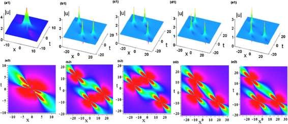
  Second-order rogue wave solution $\pmb{\tilde{u}_{2}}$ with $\pmb{c=\alpha=\beta=1}$ given by Eq. ( 32 ) at different values of $\pmb{b_{1}}$ , $\pmb{d_{1}}$ . (a1)-(a2) $b_{1}=d_{1}=0$; (b1)-(b2) $b_{1}=1\text{,}000$, $d_{1}=0$; (c1)-(c2) $b_{1}=-1\text{,}000$, $d_{1}=0$; (d1)-(d2) $b_{1}=0$, $d_{1}=1\text{,}000$; (e1)-(e2) $b_{1}=d_{1}=1\text{,}000$. (Color online.)

• For solution $\tilde{u}_{2}$ with parameters $c=\alpha=\beta =1$, $d_{1}=0$, and $b_{1}\neq0$ (e.g., $b_{1}=1\text{,}000$) or $c=\alpha=\beta=1$, $b_{1}=0$, and $d_{1}\neq0$ (e.g., $d_{1}=1\text{,}000$), we see that $\tilde {u}_{2}\rightarrow1$ as $x\rightarrow\infty$ and $t\rightarrow\infty$, the second-order RW generates a weak interaction, and, at the same time, it is split into three first-order RWs with a triangle array structure (see Figure 3(b1)-(b2), (d1)-(d2)), and the triangle structure becomes larger as $|b_{1}|$ or $|d_{1}|$ increases. When $b_{1}=-1\text{,}000$ or $d_{1}=-1\text{,}000$, the triangle structure rotates 180 degrees with respect to the origin (see Figure 3(c1)-(c2)). When parameters $c=\alpha=\beta=1$ and $b_{1} d_{1}\neq0$ (e.g., $b_{1}=1\text{,}000$, $d_{1}=1\text{,}000$), the second-order RW is also split into three first-order RWs with a triangle array structure (see Figure 3(e1)-(e2)), and comparing Figure 3(e1)-(e2) with Figure 3(b1)-(b2), (d1)-(d2), we see that the triangle structure also rotates.

(III) When $N =4$, based on the generalized perturbation $(1,3)$-fold DT, we can derive the third-order RW solution with seven arbitrary constant parameters α, β, c, $b_{1}$, $d_{1}$, $b_{2}$, $d_{2}$:

$$ \tilde{u}_{3}=u_{0}+{B^{(7)}}=ce^{i[ax+(\alpha a+2\alpha\beta+\alpha \beta^{2} c^{2}+\frac{\alpha\beta^{2}}{a})t]}+ {B^{(7)}}, $$

(33)

where the determinant form of ${B^{(7)}}$ is omitted here. The analytical expression of $\tilde{u}_{3}$ with $a=-\frac{1}{c^{2}}$ is very complicated and therefore is omitted here. Next, we discuss some special structures of the third-order RW for the following four cases:

• For solution $\tilde{u}_{3}$ with parameters $c=\alpha=1$, $\beta=2$, $b_{1}=d_{1}=b_{2}=d_{2}=0$, we see that $\tilde{u}_{2}\rightarrow1$ as $x\rightarrow\infty$ and $t\rightarrow\infty$ and that the third-order RW generates a strong interaction and crowd round the origin; the corresponding wave profiles are shown in Figure 4(a1)-(a2).

  Figure 4

  

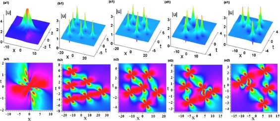
  Third-order rogue wave solution $\pmb{\tilde{u}_{3}}$ with $\pmb{c=\alpha=1}$ , $\pmb{\beta=2}$ given by Eq. ( 33 ) at different values of $\pmb{b_{i}}$ , $\pmb{d_{i}}$ ( $\pmb{i=1,2}$ ). (a1)-(a2) $b_{1}=d_{1}=b_{2}=d_{2}=0$; (b1)-(b2) $b_{1}=1\text{,}000$, $d_{1}=b_{2}=d_{2}=0$; (c1)-(c2) $b_{2}=10\text{,}000$, $b_{1}=d_{1}=d_{2}=0$; (d1)-(d2) $b_{1}=90$, $b_{2}=-1\text{,}080$, $d_{1}=d_{2}=0$; (e1)-(e2) $b_{1}=-140$, $b_{2}=2\text{,}300$, $d_{1}=d_{2}=0$. (Color online.)

• For solution $\tilde{u}_{3}$ with parameters $c=\alpha=1$, $\beta=2$, $d_{1}=b_{2}=d_{2}=0$, $b_{1}\neq0$ (e.g., $b_{1}=1\text{,}000$) or $c=\alpha=\beta =1$, $b_{1}=b_{2}=d_{2}=0$, $d_{1}\neq0$ (see Figure 4(b1)-(b2)), we see that $\tilde{u}_{3}\rightarrow1$ as $x\rightarrow\infty$ and $t\rightarrow \infty$, the third-order RW generates a weak interaction, and, at the same time, it is split into six first-order RWs with a regular triangle array structure, and the triangle structure becomes larger as $|b_{1}|$ or $|d_{1}|$ increases.

• For solution $\tilde{u}_{3}$ with parameters $c=\alpha =1$, $\beta=2$, $b_{1}=d_{1}=d_{2}=0$, $b_{2}\neq0$ (e.g., $b_{2}=10\text{,}000$) or $c=\alpha =\beta=1$, $b_{1}=d_{1}=b_{2}=0$, $d_{2}\neq0$ (see Figure 4(c1)-(c2)), we see that $\tilde{u}_{3}\rightarrow1$ as $x\rightarrow\infty$ and $t\rightarrow\infty$, the third-order RW generate the weak interaction, and, at the same time, the third-order RW is split into six first-order RWs with a regular pentagon array structure, and the pentagon structure becomes larger as $|b_{2}|$ or $|d_{2}|$ increases.

• For solution $\tilde{u}_{3}$ with parameters $c=\alpha=\beta =1$ and $b_{1} b_{2}\neq0$, $d_{1}=d_{2}=0$ or $b_{1} d_{2}\neq0$, $d_{1}=b_{2}=0$ or $d_{1} b_{2}\neq0$, $b_{1}=d_{2}=0$ or $d_{1} d_{2}\neq0$, $b_{1}=b_{2}=0$, solution $\tilde {u}_{3}\rightarrow1$ as $x\rightarrow\infty$ and $t\rightarrow\infty$, the third-order RW may be split into six first-order RWs (or one second-order RW and three first-order RWs or two second-order RWs) with a static irregular array structure. When $c=\alpha=1$, $\beta=2$, $b_{1}=90$, $b_{2}=-1\text{,}080$, $d_{1}=d_{2}=0$ or $c=\alpha=1$, $\beta=2$, $b_{1}=-140$, $b_{2}=2\text{,}300$, $d_{1}=d_{2}=0$, the third-order RW with weak interaction has an irregular structure; the corresponding wave profiles are shown in Figure 4(d1)-(d2), (e1)-(e2). However, it is obvious that the influences for two sets of parameters are different through comparing Figure 4(d1)-(d2) with Figure 4(e1)-(e2); different parameters can change the space arrangement of the third-order RW.

With the aid of symbolic computation Maple, solutions (30), (32) and (33) have been verified by substituting them into Eq. (1).

6 Conclusions

Equation (1) can model nonlinear pulse propagation in monomode optical fibers. In this paper, we have constructed the perturbation $(n;N-n)$-fold DT for Eq. (1). As an application, the generalized perturbation $(1,N-1)$-fold DT method with the same one spectral parameter allows us to calculate the higher-order RWs in terms of determinants for Eq. (1) in a unified way without complicated iteration procedure. Specifically, the first-, second-, and third-order RW structures are shown graphically: Figure 2 shows the first-order RW structures with $N=2$; Figure 3 exhibits the second-order RW interaction structures with $N=3$; Figure 4 exhibits the third-order RW interaction structures with $N=4$. Solutions and figures obtained in this paper might be helpful for understanding physical phenomena in optical fibers described by Eq. (1). We hope that our results are useful for understanding the generation mechanism and finding possible application of RWs. We believe that the method in this paper can be generalized to seek for some other types of nonlinear wave models, and we will carry out a further investigation in the future.

Appendix

$$\begin{aligned}& \phi^{(1)}= -\frac{1}{8}e^{\frac{i}{2}(-x-t\alpha+2 t\alpha\beta)}\sqrt {2}\bigl(- 2 i t^{2} \alpha^{2}-4 t \alpha+2 t^{2} \alpha^{2}+2 x^{2}+1+i+4 x t \alpha \\& \hphantom{\phi^{(1)}={}}{}- 4 i x t \alpha- 4 i x t \alpha\beta^{2}+ 4 i t \alpha\beta^{2}-2 t^{2} \alpha^{2} \beta^{4}-4 x+ 2 i \alpha^{2} \beta^{4} t^{2} \\& \hphantom{\phi^{(1)}={}}{}- 4 i t^{2} \alpha^{2} \beta ^{2}-4 x t \alpha\beta^{2}-4 \alpha^{2} \beta^{2} t^{2}- 2 i x^{2}\bigr) , \\& \psi^{(1)}= \frac{i}{8}e^{-\frac{i}{2}(-x-t\alpha+2 t\alpha\beta)} \sqrt{2}\bigl(2 x^{2}+4 x- 2 i t^{2} \alpha^{2}+1+i \\& \hphantom{\psi^{(1)}={}}{}- 4 i x t \alpha+4 t \alpha+2 t^{2} \alpha^{2}- 4 i t \alpha \beta^{2}-4 x t \alpha\beta^{2}-4 \alpha^{2} \beta ^{2} t^{2} \\& \hphantom{\psi^{(1)}={}}{}- 4 i x t \alpha\beta^{2}+ 2 i \alpha^{2} \beta^{4} t^{2}+4 x t \alpha- 4 i t^{2} \alpha^{2} \beta^{2}- 2 i x^{2}-2 t^{2} \alpha^{2} \beta^{4}\bigr) , \\& \phi^{(2)}= -\frac{1}{192}e^{\frac{i}{2}(-x-t\alpha+2 t\alpha\beta )}\sqrt{2}\bigl(-12+48 t^{2} \alpha^{2} \beta^{2}+60 x-24 x t \alpha+8 i t^{3} \alpha ^{3} \beta^{6}+8 t^{3} \alpha^{3} \\& \hphantom{\phi^{(2)}={}}{}+36 i t \alpha\beta^{2}-24 t^{3} \alpha^{3} \beta ^{2}+8 t^{3} \alpha^{3} \beta^{6}+24 x^{2} t \alpha+24 x t^{2} \alpha^{2}-24 t^{3} \alpha^{3} \beta^{4}+48 b_{1} \\& \hphantom{\phi^{(2)}={}}{}-48 i x t^{3} \alpha^{3} \beta^{4}+240 i x t \alpha-24 x t^{2} \alpha^{2} \beta^{4}-24 x^{2} t \alpha\beta^{2}-48 x t^{2} \alpha^{2} \beta ^{2}+12 \alpha \beta^{2} t \\& \hphantom{\phi^{(2)}={}}{}+60 t \alpha-12 x^{2}-12 t^{2} \alpha^{2}+48 x t \alpha \beta^{2}+48 t \alpha \beta^{2} b_{1}-48 t \alpha\beta^{2} d_{1}+48 x^{2} t^{2} \alpha^{2} \beta^{2} \\& \hphantom{\phi^{(2)}={}}{}+48 x t^{3} \alpha^{3} \beta^{2}-16 t^{3} \alpha^{3} \beta^{6} x+16 x^{3} t \alpha\beta^{2}-48 b_{1} x-48 x d_{1}-48 t \alpha b_{1}-48 t \alpha d_{1} \\& \hphantom{\phi^{(2)}={}}{}+12 t^{2} \alpha^{2} \beta^{4}+16 t^{4} \alpha^{4} \beta^{2}-16 t^{4} \alpha^{4} \beta^{6}+120 i x^{2}-24 i x^{2} t^{2} \alpha^{2} \beta^{4}+48 i t \alpha\beta^{2} d_{1} \\& \hphantom{\phi^{(2)}={}}{}-48 i x t^{2} \alpha^{2} \beta^{2}-24 i x^{2} t \alpha\beta^{2}-24 i t^{4} \alpha^{4} \beta^{4}+24 i t^{2} \alpha^{2} \beta^{2}-24 i x t^{2} \alpha^{2}+8 x^{3} \\& \hphantom{\phi^{(2)}={}}{}-24 i x^{2} t \alpha+48 i d_{1}+48 i t \alpha\beta^{2} b_{1}+4 i x^{4}+24 i x^{2} t^{2} \alpha^{2}+48 i t \alpha b_{1}+24 i x t \alpha\beta^{2} \\& \hphantom{\phi^{(2)}={}}{}+24 i x t^{2} \alpha^{2} \beta^{4}+24 i t^{3} \alpha^{3} \beta^{4}-8 i x^{3}+15 i-84 i x+72 i t^{2} \alpha^{2} \beta^{4}-48 i t \alpha d_{1} \\& \hphantom{\phi^{(2)}={}}{}-24 i t^{3} \alpha^{3} \beta^{2}+16 i x^{3} t \alpha+4 i t^{4} \alpha^{4} \beta^{8}+120 i t^{2} \alpha^{2}+48 i b_{1} x+4 i t^{4} \alpha ^{4} \\& \hphantom{\phi^{(2)}={}}{}-84 i t \alpha-8 i t^{3} \alpha^{3}-48 i x d_{1}+16 i t^{3} \alpha^{3} x\bigr) , \\& \psi^{(2)}=\frac{i}{192}e^{-\frac{i}{2}(-x-t\alpha+2 t\alpha\beta )}\sqrt{2}\bigl(-12+48 t^{2} \alpha^{2} \beta^{2}-60 x-24 x t \alpha-8 t^{3} \alpha ^{3}+24 t^{3} \alpha^{3} \beta^{2} \\& \hphantom{\psi^{(2)}={}}{}-8 t^{3} \alpha^{3} \beta^{6}-24 x^{2} t \alpha-24 x t^{2} \alpha^{2}+24 t^{3} \alpha^{3} \beta^{4}-48 b_{1}-36 i t \alpha\beta^{2}+16 i t^{3} \alpha^{3} x \\& \hphantom{\psi^{(2)}={}}{}+24 x t^{2} \alpha^{2} \beta^{4}+24 x^{2} t \alpha\beta^{2}+48 x t^{2} \alpha^{2} \beta^{2}-12 \alpha\beta^{2} t-60 t \alpha-12 x^{2}-12 t^{2} \alpha^{2} \\& \hphantom{\psi^{(2)}={}}{}+48 x t \alpha \beta^{2}+48 t \alpha\beta^{2} b_{1}-48 t \alpha \beta ^{2} d_{1}+48 x^{2} t^{2} \alpha^{2} \beta^{2}+48 x t^{3} \alpha^{3} \beta^{2}-16 t^{3} \alpha^{3} \beta^{6} x \\& \hphantom{\psi^{(2)}={}}{}+16 x^{3} t \alpha\beta^{2}-48 b_{1} x-48 x d_{1}-48 t \alpha b_{1}-48 t \alpha d_{1}+12 t^{2} \alpha^{2} \beta^{4}+16 t^{4} \alpha^{4} \beta ^{2} \\& \hphantom{\psi^{(2)}={}}{}-16 t^{4} \alpha^{4} \beta^{6}-24 i x t^{2} \alpha^{2} \beta^{4}+24 i x^{2} t \alpha +48 i t \alpha \beta^{2} b_{1}-48 i t \alpha d_{1}+48 i t \alpha b_{1} \\& \hphantom{\psi^{(2)}={}}{}+24 i t^{3} \alpha^{3} \beta^{2}-24 i x^{2} t^{2} \alpha^{2} \beta^{4}+120 i t^{2} \alpha^{2}+48 i b_{1} x-24 i t^{3} \alpha^{3} \beta^{4}+240 i x t \alpha \\& \hphantom{\psi^{(2)}={}}{}+48 i x t^{2} \alpha^{2} \beta^{2}+72 i t^{2} \alpha^{2} \beta^{4}+120 i x^{2}-48 i x t^{3} \alpha^{3} \beta ^{4}+24 i t^{2} \alpha^{2} \beta^{2}+16 i x^{3} t \alpha \\& \hphantom{\psi^{(2)}={}}{}+8 i x^{3}-8 x^{3}-8 i t^{3} \alpha^{3} \beta^{6}+48 i t \alpha\beta^{2} d_{1}+84 i x-48 i d_{1}+24 i x t^{2} \alpha^{2} \\& \hphantom{\psi^{(2)}={}}{}+15 i+24 i x^{2} t \alpha\beta^{2}+4 i t^{4} \alpha^{4} \beta^{8}+84 i t \alpha-24 i t^{4} \alpha^{4} \beta^{4}+24 i x^{2} t^{2} \alpha^{2}+4 i x^{4} \\& \hphantom{\psi^{(2)}={}}{}+4 i t^{4} \alpha^{4}-48 i x d_{1}+8 i t^{3} \alpha^{3}+24 i x t \alpha \beta^{2}\bigr) , \\& \phi^{(3)}= -\frac{1}{23\text{,}040}e^{\frac{i}{2}(-x-t\alpha+2 t\alpha\beta )}\sqrt{2}\bigl(-405-1\text{,}440 x^{2} d_{1}-1\text{,}440 b_{1} x^{2}-5\text{,}760 i x d_{2} \\& \hphantom{\phi^{(3)}={}}{}+8 t^{6} \alpha^{6} \beta^{1}2-48 t^{6} \alpha^{6} \beta^{2}+48 i t^{5} \alpha^{5}-8\text{,}100 t^{2} \alpha^{2} \beta^{2}-6\text{,}840 x^{2} t^{2} \alpha^{2}+2\text{,}880 x \\& \hphantom{\phi^{(3)}={}}{}-120 t^{6} \alpha^{6} \beta^{8}-1\text{,}440 i b_{1}^{2}+1\text{,}440 i d_{1}^{2}+3\text{,}840 i x^{3}-8 i x^{6}-17\text{,}010 i x^{2}-1\text{,}260 i x^{4} \\& \hphantom{\phi^{(3)}={}}{}+5\text{,}760 i d_{2}+48 i x^{5}-1\text{,}440 i t \alpha \beta^{2} b_{1}-5\text{,}760 t \alpha b_{2}-4\text{,}560 x t^{3} \alpha^{3}+5\text{,}760 i b_{2} x \\& \hphantom{\phi^{(3)}={}}{}-120 t^{4} \alpha^{4} x^{2}+1\text{,}080 t^{4} \alpha^{4} \beta^{4}+48 i t^{5} \alpha^{5} \beta^{1}0 x-2\text{,}880 i x t^{2} \alpha^{2} b_{1}-25\text{,}380 x t \alpha \\& \hphantom{\phi^{(3)}={}}{}-17\text{,}010 i t^{2} \alpha^{2}-1\text{,}440 i x^{2} d_{1}+240 t^{3} \alpha^{3}-2\text{,}880 i x d_{1} t \alpha+1\text{,}440 i t^{2} \alpha^{2} \beta^{4} d_{1} \\& \hphantom{\phi^{(3)}={}}{}+2\text{,}880 i t^{3} \alpha^{3} \beta^{4} b_{1}-2\text{,}880 i t^{3} \alpha^{3} d_{1} \beta^{2}+2\text{,}880 i t^{2} \alpha^{2} \beta^{4} b_{1} x-2\text{,}880 i x^{2} t \alpha b_{1} \\& \hphantom{\phi^{(3)}={}}{}-2\text{,}880 i x^{2} t \alpha\beta^{2} d_{1}-5\text{,}760 i x d_{1} t^{2} \alpha^{2} \beta^{2}-720 i x^{2} t \alpha\beta^{2}-1\text{,}440 i x t^{2} \alpha^{2} \beta^{2} \\& \hphantom{\phi^{(3)}={}}{}+2\text{,}880 i d_{1} b_{1}-480 i t^{4} \alpha^{4} \beta^{6} x^{2}+480 i x^{2} t^{4} \alpha^{4} \beta^{2}+240 i t^{5} \alpha^{5} \beta^{2} x+240 i x^{4} t^{2} \alpha^{2} \beta^{2} \\& \hphantom{\phi^{(3)}={}}{}+1\text{,}200 i t^{3} \alpha^{3} \beta^{6} x-120 i t^{4} \alpha^{4} \beta^{8} x^{2}+480 i x t^{5} \alpha^{5} \beta^{4}+720 i x^{2} t^{4} \alpha^{4} \beta^{4} \\& \hphantom{\phi^{(3)}={}}{}+480 i x^{3} t^{3} \alpha^{3} \beta^{4}+48 i x^{5} t \alpha\beta^{2}+5\text{,}220 i x t \alpha \beta^{2}+7\text{,}920 i x t^{3} \alpha^{3} \beta^{2}+7\text{,}920 i x^{2} t^{2} \alpha^{2} \beta ^{2} \\& \hphantom{\phi^{(3)}={}}{}+2\text{,}640 i x^{3} t \alpha\beta^{2}+120 i x^{4} t^{2} \alpha^{2} \beta^{4}-240 i t^{5} \alpha^{5} \beta^{8} x-480 i x^{3} t^{2} \alpha^{2} \beta^{4} \\& \hphantom{\phi^{(3)}={}}{}+240 i t^{4} \alpha^{4} \beta^{8} x-14\text{,}400 i b_{1} x-1\text{,}440 i x t^{4} \alpha^{4} \beta^{4}-1\text{,}440 i x^{2} t^{3} \alpha^{3} \beta^{4}-4\text{,}560 x^{3} t \alpha \\& \hphantom{\phi^{(3)}={}}{}+2\text{,}880 i b_{1} x t \alpha\beta^{2}+2\text{,}880 i t^{2} \alpha^{2} b_{1} \beta^{2}+5\text{,}760 t^{3} \alpha^{3} \beta^{2}+1\text{,}920 t^{3} \alpha^{3} \beta^{6}+720 x^{2} t \alpha \\& \hphantom{\phi^{(3)}={}}{}+720 x t^{2} \alpha^{2}-720 t^{3} \alpha^{3} \beta ^{4}+13\text{,}140 i x-3\text{,}600 b_{1}-5\text{,}040 d_{1}+5\text{,}760 b_{2} \\& \hphantom{\phi^{(3)}={}}{}-5\text{,}760 t \alpha d_{2}-960 i x^{3} b_{1}-160 i t^{3} \alpha^{3} \beta^{6} x^{3}-8 i t^{6} \alpha^{6}+1\text{,}800 i x^{2} t^{2} \alpha^{2} \beta^{4} \\& \hphantom{\phi^{(3)}={}}{}+1\text{,}440 i b_{1} x^{2}+3\text{,}840 i t^{3} \alpha^{3}-720 x t^{2} \alpha^{2} \beta^{4}+5\text{,}760 x^{2} t \alpha \beta^{2}+11\text{,}520 x t^{2} \alpha^{2} \beta^{2} \\& \hphantom{\phi^{(3)}={}}{}+1\text{,}620 \alpha\beta^{2} t+1\text{,}440 i x d_{1}+2\text{,}880 t \alpha-1\text{,}260 i t^{4} \alpha^{4}-12\text{,}690 x^{2}-12\text{,}690 t^{2} \alpha^{2} \\& \hphantom{\phi^{(3)}={}}{}-120 x^{4} t^{2} \alpha^{2}+11\text{,}520 i x^{2} t \alpha-8\text{,}100 x t \alpha \beta^{2}-2\text{,}880 t \alpha\beta^{2} b_{1}+1\text{,}440 t \alpha\beta^{2} d_{1} \\& \hphantom{\phi^{(3)}={}}{}-9\text{,}360 x^{2} t^{2} \alpha^{2} \beta^{2}-9\text{,}360 x t^{3} \alpha^{3} \beta^{2}+2\text{,}160 t^{3} \alpha^{3} \beta^{4} x-720 t^{3} \alpha^{3} \beta^{6} x-3\text{,}120 x^{3} t \alpha\beta ^{2} \\& \hphantom{\phi^{(3)}={}}{}+1\text{,}080 x^{2} t^{2} \alpha^{2} \beta^{4}-1\text{,}140 t^{4} \alpha^{4}+1\text{,}440 b_{1} x+14\text{,}400 x d_{1}-1\text{,}140 x^{4}+780 t^{4} \alpha^{4} \beta^{8} \\& \hphantom{\phi^{(3)}={}}{}+1\text{,}440 t \alpha b_{1}+14\text{,}400 t \alpha d_{1}+4\text{,}050 t^{2} \alpha^{2} \beta^{4}-3\text{,}120 t^{4} \alpha^{4} \beta^{2}-720 t^{4} \alpha ^{4} \beta^{6} \\& \hphantom{\phi^{(3)}={}}{}+240 i t^{3} \alpha^{3} \beta^{6}-720 i t^{3} \alpha^{3} \beta^{2}+240 i x^{4} t \alpha+13\text{,}140 i t \alpha+11\text{,}520 i x t^{2} \alpha^{2} \\& \hphantom{\phi^{(3)}={}}{}-2\text{,}880 x t \alpha \beta^{2} d_{1}-1\text{,}440 i t^{2} \alpha^{2} d_{1}+480 i x^{3} t^{2} \alpha^{2}+480 i t^{3} \alpha^{3} x^{2}+240 i t^{5} \alpha^{5} \beta^{8} \\& \hphantom{\phi^{(3)}={}}{}-5\text{,}040 i t^{3} \alpha^{3} x-34\text{,}020 i x t \alpha-5\text{,}040 i x^{3} t \alpha+2\text{,}610 i t^{2} \alpha^{2} \beta^{4}+1\text{,}440 i t \alpha d_{1} \\& \hphantom{\phi^{(3)}={}}{}+660 i t^{4} \alpha^{4} \beta^{8}-7\text{,}560 i x^{2} t^{2} \alpha^{2}-1\text{,}440 t^{2} \alpha^{2} b_{1}+240 t^{5} \alpha^{5} \beta^{2}-480 t^{5} \alpha^{5} \beta^{6} \\& \hphantom{\phi^{(3)}={}}{}+48 t^{5} \alpha^{5} \beta^{1}0-1\text{,}440 t^{2} \alpha^{2} d_{1}+960 x^{3} d_{1}-5\text{,}760 b_{2} x-5\text{,}760 x d_{2}+2\text{,}880 d_{1} b_{1} \\& \hphantom{\phi^{(3)}={}}{}+1\text{,}440 b_{1}^{2}-8 x^{6}-1\text{,}440 d_{1}^{2}+5\text{,}760 t \alpha\beta^{2} b_{2}-5\text{,}760 t \alpha\beta^{2} d_{2}+2\text{,}880 x^{2} t \alpha d_{1} \\& \hphantom{\phi^{(3)}={}}{}+2\text{,}880 x t^{2} \alpha^{2} d_{1}-2\text{,}880 t^{3} \alpha^{3} \beta^{4} d_{1}-2\text{,}880 t^{3} \alpha^{3} \beta^{2} b_{1}+960 t^{3} \alpha^{3} \beta^{6} b_{1}-48 x^{5} t \alpha \beta^{2} \\& \hphantom{\phi^{(3)}={}}{}+160 t^{6} \alpha^{6} \beta ^{6}-160 t^{3} \alpha^{3} x^{3}-48 t^{5} \alpha^{5} x-48 t^{6} \alpha^{6} \beta^{1}0+960 t^{3} \alpha^{3} d_{1}-48 x^{5} t \alpha \\& \hphantom{\phi^{(3)}={}}{}+120 t^{6} \alpha^{6} \beta^{4}-2\text{,}880 x^{2} t \alpha\beta^{2} b_{1}-5\text{,}760 x t^{2} \alpha^{2} \beta^{2} b_{1}-2\text{,}880 x t^{2} \alpha^{2} \beta^{4} d_{1}-8 t^{6} \alpha^{6} \\& \hphantom{\phi^{(3)}={}}{}-240 t^{5} \alpha^{5} \beta^{2} x+480 t^{5} \alpha^{5} \beta^{6} x-240 x^{4} t^{2} \alpha^{2} \beta^{2}-480 x^{3} t^{3} \alpha^{3} \beta^{2}+480 x^{3} t^{3} \alpha^{3} \beta^{4} \\& \hphantom{\phi^{(3)}={}}{}-480 x^{2} t^{4} \alpha^{4} \beta^{2}+720 x^{2} t^{4} \alpha ^{4} \beta^{4}+480 x t^{5} \alpha^{5} \beta^{4}+160 t^{3} \alpha^{3} \beta^{6} x^{3}+480 t^{4} \alpha^{4} \beta^{6} x^{2} \\& \hphantom{\phi^{(3)}={}}{}-120 t^{4} \alpha^{4} \beta^{8} x^{2}-240 t^{5} \alpha^{5} \beta^{8} x+120 x^{4} t^{2} \alpha^{2} \beta^{4}-48 t^{5} \alpha^{5} \beta^{1}0 x-14\text{,}400 i t \alpha b_{1} \\& \hphantom{\phi^{(3)}={}}{}-960 i t^{3} \alpha^{3} b_{1}+3\text{,}600 i x t^{3} \alpha^{3} \beta^{4}+480 i x^{3} t^{3} \alpha^{3} \beta^{2}+5\text{,}220 i t^{2} \alpha^{2} \beta^{2}-48 i x^{5} t \alpha \\& \hphantom{\phi^{(3)}={}}{}+5\text{,}760 i t \alpha b_{2}-160 i t^{3} \alpha^{3} x^{3}-120 i t^{4} \alpha^{4} x^{2}-120 i x^{4} t^{2} \alpha^{2}-48 i t^{5} \alpha^{5} x-120 i t^{6} \alpha^{6} \beta^{8} \\& \hphantom{\phi^{(3)}={}}{}+120 i t^{6} \alpha^{6} \beta^{4}+240 x^{4} t \alpha\beta^{2}-2\text{,}880 x t \alpha b_{1}-2\text{,}880 t^{2} \alpha^{2} \beta^{2} d_{1}+8 i t^{6} \alpha^{6} \beta^{1}2 \\& \hphantom{\phi^{(3)}={}}{}+1\text{,}200 i t^{4} \alpha^{4} \beta^{6}+2\text{,}640 i t^{4} \alpha^{4} \beta^{2}-160 i t^{6} \alpha^{6} \beta^{6}+48 i t^{6} \alpha^{6} \beta^{2}-480 i t^{5} \alpha^{5} \beta^{4} \\& \hphantom{\phi^{(3)}={}}{}+240 i t^{4} \alpha^{4} x+1\text{,}800 i t^{4} \alpha^{4} \beta^{4}-5\text{,}760 i t \alpha d_{2}+48 i t^{6} \alpha^{6} \beta ^{1}0+1\text{,}440 i t^{2} \alpha^{2} b_{1} \\& \hphantom{\phi^{(3)}={}}{}+240 x^{3}+2\text{,}880 i t^{2} \alpha^{2} \beta^{2} d_{1}+2\text{,}880 i x t \alpha\beta^{2} d_{1}-1\text{,}440 i t^{2} \alpha^{2} \beta^{4} b_{1}+1\text{,}440 t^{2} \alpha^{2} \beta^{4} b_{1} \\& \hphantom{\phi^{(3)}={}}{}-2\text{,}880 x t \alpha d_{1}+2\text{,}880 t^{2} \alpha^{2} \beta^{2} b_{1}+1\text{,}440 t^{2} \alpha^{2} \beta^{4} d_{1}+960 x^{3} t^{2} \alpha^{2} \beta^{2} \\& \hphantom{\phi^{(3)}={}}{}+1\text{,}440 x^{2} t^{3} \alpha^{3} \beta^{2}+960 x t^{4} \alpha^{4} \beta^{2}-480 t^{3} \alpha^{3} \beta ^{6} x^{2}-960 t^{4} \alpha^{4} \beta^{6} x-3\text{,}600 i d_{1} \\& \hphantom{\phi^{(3)}={}}{}-2\text{,}880 i t \alpha\beta^{2} d_{1}+5\text{,}760 i t \alpha\beta^{2} b_{2}+2\text{,}880 i b_{1} x t \alpha-1\text{,}395 i+5\text{,}040 i b_{1} \\& \hphantom{\phi^{(3)}={}}{}+2\text{,}880 x t \alpha \beta^{2} b_{1}+960 i t^{3} \alpha^{3} \beta^{6} d_{1}-480 i t^{5} \alpha^{5} \beta^{6} x+5\text{,}760 i t \alpha\beta^{2} d_{2}\bigr) , \\& \psi^{(3)}= \frac{i}{23\text{,}040}e^{-\frac{i}{2}(-x-t\alpha+2 t\alpha\beta )}\sqrt{2}\bigl(-405+720 i t^{3} \alpha^{3} \beta^{2}+1\text{,}440 x^{2} d_{1}+1\text{,}440 b_{1} x^{2} \\& \hphantom{\psi^{(3)}={}}{}+8 t^{6} \alpha^{6} \beta^{1}2-48 t^{6} \alpha^{6} \beta^{2}-8\text{,}100 t^{2} \alpha^{2} \beta ^{2}-6\text{,}840 x^{2} t^{2} \alpha^{2}-2\text{,}880 x \\& \hphantom{\psi^{(3)}={}}{}+480 i x^{3} t^{2} \alpha^{2} \beta^{4}-120 t^{6} \alpha^{6} \beta^{8}-1\text{,}440 i b_{1}^{2}-5\text{,}760 i x d_{1} t^{2} \alpha^{2} \beta^{2}-5\text{,}760 i x d_{2} \\& \hphantom{\psi^{(3)}={}}{}-5\text{,}760 t \alpha b_{2}-4\text{,}560 x t^{3} \alpha^{3}+2\text{,}880 i d_{1} b_{1}-2\text{,}880 i x t^{2} \alpha^{2} b_{1}-120 t^{4} \alpha^{4} x^{2} \\& \hphantom{\psi^{(3)}={}}{}+1\text{,}080 t^{4} \alpha^{4} \beta^{4}-25\text{,}380 x t \alpha+7\text{,}920 i x t^{3} \alpha^{3} \beta^{2}+48 i t^{5} \alpha^{5} \beta^{1}0 x-17\text{,}010 i t^{2} \alpha^{2} \\& \hphantom{\psi^{(3)}={}}{}-240 t^{3} \alpha^{3}-2\text{,}880 i x t \alpha \beta^{2} d_{1}-1\text{,}260 i x^{4}-4\text{,}560 x^{3} t \alpha-5\text{,}760 t^{3} \alpha^{3} \beta^{2} \\& \hphantom{\psi^{(3)}={}}{}-1\text{,}920 t^{3} \alpha^{3} \beta ^{6}-720 x^{2} t \alpha-720 x t^{2} \alpha^{2}+720 t^{3} \alpha^{3} \beta^{4}+5\text{,}760 i t \alpha b_{2}+3\text{,}600 b_{1} \\& \hphantom{\psi^{(3)}={}}{}+5\text{,}040 d_{1}-5\text{,}760 b_{2}-5\text{,}760 t \alpha d_{2}+5\text{,}760 i b_{2} x+1\text{,}800 i x^{2} t^{2} \alpha^{2} \beta^{4}-5\text{,}040 i x^{3} t \alpha \\& \hphantom{\psi^{(3)}={}}{}-240 i t^{5} \alpha ^{5} \beta^{8}-160 i t^{3} \alpha^{3} \beta^{6} x^{3}-2\text{,}880 i t \alpha \beta^{2} d_{1}-5\text{,}040 i t^{3} \alpha^{3} x-1\text{,}440 i t \alpha\beta^{2} b_{1} \\& \hphantom{\psi^{(3)}={}}{}+720 x t^{2} \alpha ^{2} \beta^{4}-5\text{,}760 x^{2} t \alpha \beta^{2}-11\text{,}520 x t^{2} \alpha^{2} \beta^{2}-1\text{,}620 \alpha\beta^{2} t-2\text{,}880 t \alpha-8 i t^{6} \alpha^{6} \\& \hphantom{\psi^{(3)}={}}{}-12\text{,}690 x^{2}-12\text{,}690 t^{2} \alpha^{2}-120 x^{4} t^{2} \alpha^{2}+120 i x^{4} t^{2} \alpha^{2} \beta^{4}+240 i t^{5} \alpha^{5} \beta^{2} x \\& \hphantom{\psi^{(3)}={}}{}-8\text{,}100 x t \alpha \beta^{2}-2\text{,}880 t \alpha\beta^{2} b_{1}+1\text{,}440 t \alpha\beta^{2} d_{1}-9\text{,}360 x^{2} t^{2} \alpha^{2} \beta^{2}-9\text{,}360 x t^{3} \alpha^{3} \beta^{2} \\& \hphantom{\psi^{(3)}={}}{}+2\text{,}160 t^{3} \alpha^{3} \beta^{4} x-720 t^{3} \alpha^{3} \beta^{6} x-3\text{,}120 x^{3} t \alpha\beta^{2}+1\text{,}080 x^{2} t^{2} \alpha^{2} \beta^{4}-1\text{,}140 t^{4} \alpha^{4} \\& \hphantom{\psi^{(3)}={}}{}+1\text{,}440 b_{1} x+14\text{,}400 x d_{1}-1\text{,}140 x^{4}+780 t^{4} \alpha^{4} \beta^{8}+1\text{,}440 t \alpha b_{1}+14\text{,}400 t \alpha d_{1} \\& \hphantom{\psi^{(3)}={}}{}+4\text{,}050 t^{2} \alpha^{2} \beta^{4}-3\text{,}120 t^{4} \alpha^{4} \beta^{2}-720 t^{4} \alpha^{4} \beta^{6}+2\text{,}880 x t \alpha\beta^{2} d_{1}-480 i t^{5} \alpha^{5} \beta^{6} x \\& \hphantom{\psi^{(3)}={}}{}-160 i t^{3} \alpha^{3} x^{3}+1\text{,}440 i x t^{2} \alpha^{2} \beta^{2}-1\text{,}440 i b_{1} x^{2}-48 i t^{5} \alpha^{5}+1\text{,}440 t^{2} \alpha^{2} b_{1} \\& \hphantom{\psi^{(3)}={}}{}-240 t^{5} \alpha^{5} \beta^{2}+480 t^{5} \alpha^{5} \beta^{6}-48 t^{5} \alpha^{5} \beta^{1}0+1\text{,}440 t^{2} \alpha^{2} d_{1}+960 x^{3} d_{1}-5\text{,}760 b_{2} x \\& \hphantom{\psi^{(3)}={}}{}-5\text{,}760 x d_{2}+2\text{,}880 d_{1} b_{1}+1\text{,}440 b_{1}^{2}-8 x^{6}-1\text{,}440 d_{1}^{2}+5\text{,}760 t \alpha\beta^{2} b_{2} \\& \hphantom{\psi^{(3)}={}}{}-5\text{,}760 t \alpha\beta^{2} d_{2}+2\text{,}880 x^{2} t \alpha d_{1}+2\text{,}880 x t^{2} \alpha^{2} d_{1}-2\text{,}880 t^{3} \alpha^{3} \beta^{4} d_{1} \\& \hphantom{\psi^{(3)}={}}{}-2\text{,}880 t^{3} \alpha^{3} \beta^{2} b_{1}+960 t^{3} \alpha^{3} \beta^{6} b_{1}-48 x^{5} t \alpha \beta^{2}+160 t^{6} \alpha^{6} \beta^{6}-160 t^{3} \alpha^{3} x^{3} \\& \hphantom{\psi^{(3)}={}}{}-48 t^{5} \alpha^{5} x-48 t^{6} \alpha^{6} \beta^{1}0+960 t^{3} \alpha ^{3} d_{1} -48 x^{5} t \alpha+120 t^{6} \alpha^{6} \beta^{4}-2\text{,}880 x^{2} t \alpha\beta ^{2} b_{1} \\& \hphantom{\psi^{(3)}={}}{}-5\text{,}760 x t^{2} \alpha^{2} \beta^{2} b_{1}-2\text{,}880 x t^{2} \alpha^{2} \beta^{4} d_{1}-8 t^{6} \alpha^{6}-240 t^{5} \alpha^{5} \beta^{2} x+480 t^{5} \alpha^{5} \beta^{6} x \\& \hphantom{\psi^{(3)}={}}{}-1\text{,}260 i t^{4} \alpha^{4}-240 x^{4} t^{2} \alpha^{2} \beta^{2}-480 x^{3} t^{3} \alpha^{3} \beta^{2}+480 x^{3} t^{3} \alpha^{3} \beta^{4}-480 x^{2} t^{4} \alpha^{4} \beta^{2} \\& \hphantom{\psi^{(3)}={}}{}+720 x^{2} t^{4} \alpha^{4} \beta^{4}+480 x t^{5} \alpha^{5} \beta^{4}+160 t^{3} \alpha^{3} \beta^{6} x^{3}+480 t^{4} \alpha^{4} \beta^{6} x^{2}-120 t^{4} \alpha^{4} \beta^{8} x^{2} \\& \hphantom{\psi^{(3)}={}}{}-240 t^{5} \alpha^{5} \beta^{8} x+120 x^{4} t^{2} \alpha^{2} \beta^{4}-48 t^{5} \alpha^{5} \beta^{1}0 x+48 i x^{5} t \alpha\beta^{2}+2\text{,}640 i x^{3} t \alpha\beta ^{2} \\& \hphantom{\psi^{(3)}={}}{}+48 i t^{6} \alpha^{6} \beta^{1}0+480 i t^{5} \alpha^{5} \beta^{4}-2\text{,}880 i t^{3} \alpha^{3} d_{1} \beta^{2}+1\text{,}440 i x t^{4} \alpha^{4} \beta^{4}-48 i x^{5} \\& \hphantom{\psi^{(3)}={}}{}-120 i t^{6} \alpha^{6} \beta^{8}-240 x^{4} t \alpha\beta^{2}+2\text{,}880 x t \alpha b_{1}+2\text{,}880 t^{2} \alpha^{2} \beta^{2} d_{1}-120 i t^{4} \alpha^{4} \beta^{8} x^{2} \\& \hphantom{\psi^{(3)}={}}{}-480 i t^{4} \alpha^{4} \beta^{6} x^{2}+7\text{,}920 i x^{2} t^{2} \alpha^{2} \beta^{2}-960 i t^{3} \alpha^{3} b_{1}+2\text{,}880 i t^{2} \alpha^{2} \beta^{4} b_{1} x-8 i x^{6} \\& \hphantom{\psi^{(3)}={}}{}-7\text{,}560 i x^{2} t^{2} \alpha^{2}+2\text{,}640 i t^{4} \alpha^{4} \beta^{2}-240 x^{3}-48 i x^{5} t \alpha+960 i t^{3} \alpha^{3} \beta^{6} d_{1} \\& \hphantom{\psi^{(3)}={}}{}+48 i t^{6} \alpha^{6} \beta^{2}+1\text{,}440 i t \alpha d_{1}-14\text{,}400 i b_{1} x-14\text{,}400 i t \alpha b_{1}+5\text{,}760 i t \alpha\beta^{2} d_{2} \\& \hphantom{\psi^{(3)}={}}{}+5\text{,}220 i x t \alpha \beta^{2}-2\text{,}880 i b_{1} x t \alpha\beta^{2}+1\text{,}440 i x^{2} t^{3} \alpha^{3} \beta^{4}-1\text{,}440 t^{2} \alpha ^{2} \beta^{4} b_{1} \\& \hphantom{\psi^{(3)}={}}{}+2\text{,}880 x t \alpha d_{1}-2\text{,}880 t^{2} \alpha^{2} \beta^{2} b_{1}-1\text{,}440 t^{2} \alpha^{2} \beta^{4} d_{1}-960 x^{3} t^{2} \alpha^{2} \beta^{2} \\& \hphantom{\psi^{(3)}={}}{}-1\text{,}440 x^{2} t^{3} \alpha^{3} \beta^{2}-960 x t^{4} \alpha^{4} \beta^{2}+480 t^{3} \alpha^{3} \beta^{6} x^{2}+960 t^{4} \alpha^{4} \beta^{6} x+480 i x t^{5} \alpha^{5} \beta^{4} \\& \hphantom{\psi^{(3)}={}}{}-120 i t^{4} \alpha^{4} x^{2}-13\text{,}140 i t \alpha+3\text{,}600 i x t^{3} \alpha^{3} \beta^{4}-2\text{,}880 i x^{2} t \alpha b_{1}+8 i t^{6} \alpha^{6} \beta^{1}2 \\& \hphantom{\psi^{(3)}={}}{}-5\text{,}040 i b_{1}-2\text{,}880 i x^{2} t \alpha \beta^{2} d_{1}-160 i t^{6} \alpha^{6} \beta^{6}-5\text{,}760 i t \alpha d_{2}-240 i t^{3} \alpha^{3} \beta^{6} \\& \hphantom{\psi^{(3)}={}}{}-13\text{,}140 i x+1\text{,}200 i t^{3} \alpha^{3} \beta^{6} x-480 i x^{3} t^{2} \alpha^{2}+1\text{,}440 i x d_{1}+1\text{,}200 i t^{4} \alpha^{4} \beta^{6} \\& \hphantom{\psi^{(3)}={}}{}-34\text{,}020 i x t \alpha -2\text{,}880 i t^{2} \alpha^{2} \beta^{2} d_{1}-1\text{,}440 i t^{2} \alpha^{2} \beta^{4} d_{1}+5\text{,}760 i t \alpha \beta^{2} b_{2} \\& \hphantom{\psi^{(3)}={}}{}-2\text{,}880 x t \alpha\beta^{2} b_{1}+480 i x^{3} t^{3} \alpha^{3} \beta^{4}+720 i x^{2} t \alpha\beta^{2}-48 i t^{5} \alpha^{5} x-11\text{,}520 i x t^{2} \alpha^{2} \\& \hphantom{\psi^{(3)}={}}{}+240 i x^{4} t^{2} \alpha^{2} \beta^{2}-2\text{,}880 i b_{1} x t \alpha-3\text{,}840 i t^{3} \alpha^{3}-3\text{,}840 i x^{3}+1\text{,}440 i t^{2} \alpha^{2} d_{1} \\& \hphantom{\psi^{(3)}={}}{}-5\text{,}760 i d_{2}+120 i t^{6} \alpha^{6} \beta^{4}+2\text{,}880 i x d_{1} t \alpha+480 i x^{3} t^{3} \alpha^{3} \beta ^{2}-2\text{,}880 i t^{2} \alpha^{2} b_{1} \beta^{2} \\& \hphantom{\psi^{(3)}={}}{}-120 i x^{4} t^{2} \alpha^{2}+660 i t^{4} \alpha^{4} \beta^{8}-480 i t^{3} \alpha^{3} x^{2}+1\text{,}440 i x^{2} d_{1}+2\text{,}880 i t^{3} \alpha ^{3} \beta^{4} b_{1} \\& \hphantom{\psi^{(3)}={}}{}+1\text{,}440 i t^{2} \alpha^{2} \beta^{4} b_{1}+480 i x^{2} t^{4} \alpha^{4} \beta^{2}-1\text{,}440 i t^{2} \alpha^{2} b_{1}-240 i t^{5} \alpha^{5} \beta^{8} x-240 i t^{4} \alpha^{4} x \\& \hphantom{\psi^{(3)}={}}{}+720 i x^{2} t^{4} \alpha^{4} \beta^{4}+1\text{,}800 i t^{4} \alpha^{4} \beta ^{4}-17\text{,}010 i x^{2}-1\text{,}395 i+1\text{,}440 i d_{1}^{2}+3\text{,}600 i d_{1} \\& \hphantom{\psi^{(3)}={}}{}-11\text{,}520 i x^{2} t \alpha-960 i x^{3} b_{1}+2\text{,}610 i t^{2} \alpha^{2} \beta^{4}-240 i t^{4} \alpha^{4} \beta^{8} x \\& \hphantom{\psi^{(3)}={}}{}-240 i x^{4} t \alpha+5\text{,}220 i t^{2} \alpha^{2} \beta^{2}\bigr) . \end{aligned}$$

References

1. Zhai, BG, Zhang, WG, Wang, XL, Zhang, HQ: Multi-rogue waves and rational solutions of the coupled nonlinear Schrödinger equations. Nonlinear Anal., Real World Appl. 14, 14-27 (2013)
Article  MathSciNet  MATH  Google Scholar
2. Guo, BL, Ling, LL, Liu, QP: Nonlinear Schrödinger equation: generalized Darboux transformation and rogue wave solutions. Phys. Rev. E 85, 026607 (2012)
Article  Google Scholar
3. Wang, DS, Chen, F, Wen, XY: Darboux transformation of the general Hirota equation: multi-soliton solutions, breather solutions and rogue wave solutions. Adv. Differ. Equ. 2016, 67 (2016)
Article  MathSciNet  Google Scholar
4. Wen, XY, Yan, ZY: Modulational instability and higher-order rogue waves with parameters modulation in a coupled integrable AB system via the generalized Darboux transformation. Chaos 25, 123115 (2015)
5. Wen, XY, Yan, ZY, Yang, YQ: Dynamics of higher-order rational solitons for the nonlocal nonlinear Schrödinger equation with the self-induced parity-time-symmetric potential. Chaos 26, 063123 (2016)
6. Yu, FJ: Nonautonomous rogue waves and ‘catch’ dynamics for the combined Hirota-LPD equation with variable coefficients. Commun. Nonlinear Sci. Numer. Simul. 34, 142-153 (2016)
7. Yu, FJ: Nonautonomous soliton, controllable interaction and numerical simulation for generalized coupled cubic-quintic nonlinear Schrödinger equations. Nonlinear Dyn. 85, 1203-1216 (2016)
8. Zhang, HQ, Chen, J: Rogue wave solutions for the higher-order nonlinear Schrödinger equation with variable coefficients by generalized Darboux transformation. Mod. Phys. Lett. B 30, 1650106 (2016)
9. Zhang, HQ, Yuan, SS, Wang, Y: Generalized Darboux transformation and rogue wave solution of the coherently-coupled nonlinear Schrödinger system. Mod. Phys. Lett. B 30, 1650208 (2016)
10. Wen, LL, Zhang, HQ: Rogue wave solutions of the \((2+1)\)-dimensional derivative nonlinear Schrödinger equation. Nonlinear Dyn. 86, 877-889 (2016)
11. Zhang, HQ, Liu, XL, Wen, LL: Soliton, breather, and rogue wave for a \((2+1)\)-dimensional nonlinear Schrödinger equation. Z. Naturforsch. A 71, 95-101 (2016)
Google Scholar
12. Geng, XG, Lv, YY: Darboux transformation for an integrable generalization of the nonlinear Schrödinger equation. Nonlinear Dyn. 69, 1621-1630 (2012)
13. Fokas, AS: On a class of physically important integrable equations. Physica D 87, 145-150 (1995)
14. Lenells, J, Fokas, AS: On a novel integrable generalization of the nonlinear Schrödinger equation. Nonlinearity 22, 11-27 (2009)
15. Yan, ZY, Dai, CQ: Optical rogue waves in the generalized inhomogeneous higher-order nonlinear Schrödinger equation with modulating coefficients. J. Opt. 15, 064012 (2013)
16. Guo, R, Hao, HQ: Breathers and multi-soliton solutions for the higher-order generalized nonlinear Schrödinger equation. Commun. Nonlinear Sci. Numer. Simul. 18, 2426-2435 (2013)
17. Geng, XG, Ham, HW: Darboux transformation and soliton solutions for generalized nonlinear Schrödinger equations. J. Phys. Soc. Jpn. 68, 1508-1542 (1999)
Article  MATH  Google Scholar
18. Li, WB, Xue, CY, Sun, LL: The general mixed nonlinear Schrödinger equation: Darboux transformation, rogue wave solutions, and modulation instability. Adv. Differ. Equ. 2016, 233 (2016)
19. Wen, XY, Hu, XY: N-Fold Darboux transformation and solitonic interactions for a Volterra lattice system. Adv. Differ. Equ. 2014, 213 (2014)
20. Wen, XY, Meng, XH, Xu, XG, Wang, JT: N-Fold Darboux transformation and explicit solutions in terms of the determinant for the three-field Blaszak-Marciniak lattice. Appl. Math. Lett. 26, 1076-1081 (2013)
Download references
Acknowledgements
The author thanks the editor and reviewers for their valuable suggestions. This work has been supported by the National Natural Science Foundation of China under Grant No. 11375030, China Postdoctoral Science Foundation under Grant No. 2015M570161, and the Beijing Natural Science Foundation under Grant No. 1153004.
Author information
Authors and Affiliations
Authors
Corresponding author
Correspondence to Xiao-Yong Wen.
Additional information
Competing interests
The author declares that he has no competing interests.
Author’s contributions
The only author has made all contributions. The author has read and approved the final manuscript.