The plethora of explicit solutions of the fractional KS equation through liquid–gas bubbles mix under the thermodynamic conditions via Atangana–Baleanu derivative operator

Abstract

Novel explicit wave solutions are constructed for the Kudryashov–Sinelshchikov (KS) equation through liquid–gas bubbles mix under the thermodynamic conditions. A new fractional definition (Atangana–Baleanu derivative operator) is employed through the modified Khater method to get new wave solutions in distinct types of this model that is used to describe the phenomena of pressure waves through liquid–gas bubbles mix under the thermodynamic conditions. The stability property of the obtained solutions is tested to show the ability of our obtained solutions through the physical experiments. The novelty and advantage of the proposed method are illustrated by applying to this model. Some sketches are plotted to show more about the dynamical behavior of this model.

1 Introduction

Nowadays, many natural phenomena have been derived in nonlinear partial differential equations with an integer order. These models are included in various and distinct branches of science such as chemistry, physics, biology, engineering, economy, etc. However, using the integer order of these models is not sufficient where the nonlocal property does not appear in these formulas so that many models have been formulated in fractional nonlinear partial differential equations specially to discover that kind of property. Studying these models gives more novel properties of them specially by using the computational and numerical schemes. For using most of these schemes, one needs fractional operators to convert the fractional formulas to nonlinear ordinary differential equations with integer order such as Caputo, Caputo–Fabrizio definition, fractional Riemann–Liouville derivatives, conformable fractional derivative, and so on [1–15]. These fractional operators have been employed to investigate the exact and numerical solutions of many phenomena. These solutions have been obtained in explicit formulas by using different analytical schemes such as [16–25].

Recently, the mK method has been formulated and applied to distinct physical models such as the $(2+1)$-dimensional KD equation, the complex Ginzburg–Landau model, KdV equation, the fractional $(N+1)$ Sinh–Gordon, biological population, equal width, modified equal width, Duffing equations, and so on [26–35].

This method depends on a new auxiliary equation, which is equal to the auxiliary equation of the main future of the modified mathematical technique [36]. The auxiliary equation of the mK method is given by

$$\begin{aligned} \mathcal{E}'(\varphi)= \frac{1}{ln (\mathcal{Q})} \bigl[ \delta \mathcal{Q}^{\mathcal{E}(\wp)}+\varrho\mathcal{Q}^{-\mathcal {E}(\wp)}+\chi \bigr], \end{aligned}$$

(1)

where δ, ϱ, χ, $\mathcal{Q}$ are arbitrary constants; whereas the auxiliary equation of the extended exponential-expansion function method is given by

$$\begin{aligned} \varPsi^{\prime 2}(\wp)=\beta_{1} \varPsi^{2}(\wp)+\beta_{2} \varPsi ^{3}(\wp)+ \beta_{3} \varPsi^{4}(\wp), \end{aligned}$$

(2)

where $\beta_{i}$ ($i=1,2,3$) are arbitrary constants. So Eqs. (1) and (2) are equal when [$\mathcal{Q}^{\mathcal {E}(\wp)}=\varPsi(\wp)$, $\varrho=0$, $\beta_{1}=\chi^{2}$, $\beta _{2}=2 \delta\chi$, $\beta_{3}=\delta^{2}$]. Using this technique leads to the equality of the mK auxiliary equation with many other analytical methods, but the mK method can obtain more solutions than most of them. This equivalence shows superiority, power, and productivity of the mK method.

In this context, the mK method is employed to construct new formulas of solutions for the fractional nonlinear KS equation, which is given by [37–43]:

$$\begin{aligned} \mathcal{D}_{x} ^{\vartheta} \mathcal{S}_{t}+ \lambda\mathcal{S} \mathcal{S}_{x}+\mathcal{S}_{x x x}-\alpha ( \mathcal{S} \mathcal{S}_{x x} )_{x}-\mu\mathcal{S}_{x} \mathcal{S}_{x x}-\beta\mathcal{S}_{x x}-\sigma (\mathcal{S} \mathcal{S}_{x} )_{x}=0, \end{aligned}$$

(3)

where [$\mathcal{S}=\mathcal{S}(x, t)$] is the function that is used to describe the dynamical behavior of the nonlinear wave processes in a liquid containing gas bubbles. Additionally, [λ, α, μ, β, σ] are arbitrary constants while [$\vartheta\in{}]0,1[$]. This equation was defined by Kudryashov and Sinelshchikov in 2010 to describe the nonlinear wave processes in a liquid containing gas bubbles. This equation is also considered as a general form of the well-known models KdV and KdV–Burger equations under the following conditions:

• For [$\mu=\alpha=\sigma=\beta=0$], Eq. (3) equals the well-known Korteweg–de Vries equation.

• For [$\alpha=\mu=\sigma=0$], Eq. (3) equals the well-known Korteweg–de Vries Burgers equation.

• For [$\lambda=\alpha=1$, $\beta=\sigma=0$], Eq. (3) equals the generalized Korteweg–de Vries equation.

1.1 Fractional $\mathcal{ABR}$ operator

The $\mathcal{ABR}$ fractional operator is given by [44–48]

$$\begin{aligned} ^{\mathcal{ABR}} \mathcal{D}^{\vartheta}_{a+} \mathcal{F}(t)=\frac {\mathcal{B}(\vartheta)}{1-\vartheta} \frac{d}{d t} \int_{a}^{t} \mathcal{F}(x) \mathcal{G}_{\vartheta} \biggl(\frac{-\vartheta (t-\vartheta)^{\vartheta}}{1-\vartheta} \biggr)\, dx, \end{aligned}$$

(4)

where $\mathcal{G}_{\vartheta}$ is the Mittag-Leffler function, defined by the following formula:

$$\mathcal{G}_{\vartheta} \biggl(\frac{-\vartheta(t-\vartheta )^{\vartheta}}{1-\vartheta} \biggr)=\sum _{n=0}^{\infty} \frac { (\frac{-\vartheta}{1-\vartheta} ) ^{n} (t-x)^{\vartheta n}}{\varGamma(\vartheta n+1)}, $$

and $\mathcal{B}(\vartheta)$ is a normalization function. Thus

$$\begin{aligned} ^{\mathcal{ABR}} \mathcal{D}^{\vartheta}_{a+} \mathcal{F}(x) =\frac {\mathcal{B}(\vartheta)}{1-\vartheta} \sum_{n=0}^{\infty} \biggl(\frac{-\vartheta}{1-\vartheta} \biggr) ^{n} {}^{R L} \mathcal {I}^{\vartheta n}_{a} \mathcal{F}(x). \end{aligned}$$

(5)

For further properties of this fractional operator, you can see [44, 49, 50]. This leads to

$$\mathcal{S}(x,t)=\mathcal{S}(\wp),\quad \wp=x+\frac{c (1-\vartheta) t^{- \vartheta n}}{B(\vartheta) \sum_{n=0}^{\infty} (-\frac {\vartheta}{1-\vartheta} )^{n} \varGamma(1-\vartheta n)}, $$

where c is an arbitrary constant. This wave transformation converts Eq. (3) to ODE. Integration of the obtained ODEs once with zero constant of the integration gives

$$\begin{aligned} c \mathcal{S}+\frac{\lambda}{2} \mathcal{S}^{2}+\mathcal {S}''-\alpha\mathcal{S} \mathcal{S}''- \frac{\mu}{2} \mathcal {S}^{\prime 2}-\beta \mathcal{S}'-\sigma\mathcal{S} \mathcal{S}'=0. \end{aligned}$$

(6)

Calculating the homogeneous balance value in Eq. (6) yields $N=2$. Thus, the general formula of solution according to the mK method is given by

$$ \begin{aligned} [b]\mathcal{S}(\wp)&=\sum _{i=1}^{N} a_{i} \mathcal{Q}^{i \mathcal{E}(\wp )}+ \sum_{i=1}^{N} b_{i} \mathcal{Q}^{-i \mathcal{E}(\wp)}+a_{0}\\ &=a_{2} \mathcal{Q}^{2 \mathcal{E}(\wp)}+ a_{1} \mathcal{Q}^{ \mathcal {E}(\wp)}+a_{0}+b_{1} \mathcal{Q}^{- \mathcal{E}(\wp)}+b_{2} \mathcal {Q}^{-2 \mathcal{E}(\wp)}, \end{aligned} $$

(7)

where $a_{0}$, $a_{1}$, $a_{2}$, $b_{1}$, $b_{2}$ are arbitrary constants.

The rest of this article is arranged in the following order. In Sect. 2 we apply the mK method to the nonlinear fractional nonlinear $(2+1)$-BLMP equation. Moreover, some sketches are given to show more physical properties of both models. Section 4 discusses the stability property of the obtained solutions. Section 5 gives the conclusion of the whole research.

2 Abundant wave solutions of the fractional KS equation

Applying the mK method with its auxiliary equation and the suggested general solutions for the fractional KS equation leads to a system of algebraic equations. Using Mathematica 11.2 to find the values of the parameters in this system leads to the following:

Family I

$$\begin{gathered} \biggl[ a_{1}\to\frac{a_{2} (\mu\chi+3 \sigma)}{\delta\mu},b_{1}\to 0,b_{2} \to0,\\ \quad\lambda\to-\frac{4 \delta^{2} (a_{0} \mu+3 )}{a_{2}}+\frac{8 \delta\mu\varrho}{3}+\frac{15 \sigma^{2}}{\mu }+ \frac{\mu\chi^{2}}{3}+6 \sigma\chi,\alpha\to-\frac{\mu}{3}, \\ \qquad\text{where } (\delta\neq0, \mu\neq0, a_{2}\neq0 ) \biggr]. \end{gathered}$$

Consequently, the closed forms of solutions for the fractional KS model are given by:

When [$\chi^{2}-4 \delta\varrho<0\text{ \& }\delta\neq0$]

$$\begin{aligned}& \begin{aligned} [b]\mathcal{S}_{1}&= a_{0}-\frac{1}{4 \delta^{2} \mu} \biggl[ a_{2} \biggl(\mu \bigl( \chi^{2}-4 \delta\varrho \bigr) \\ &\quad\times\tan^{2} \biggl( \frac {1}{2} \sqrt{4 \delta\varrho-\chi^{2}} \biggl(x- \frac{(\vartheta -1) c t^{-2 \vartheta}}{B(\vartheta) \sum_{n=0}^{\infty} (-\frac{\vartheta}{1-\vartheta} )^{n} \varGamma(1-\vartheta n)} \biggr) \biggr) \\ &\quad-6 \sigma\sqrt{4 \delta\varrho-\chi^{2}} \tan \biggl( \frac{1}{2} \sqrt{4 \delta\varrho-\chi^{2}} \biggl(x- \frac{(\vartheta-1) c t^{-2 \vartheta}}{B(\vartheta) \sum_{n=0}^{\infty} (-\frac {\vartheta}{1-\vartheta} )^{n} \varGamma(1-\vartheta n)} \biggr) \biggr)\\ &\quad+\chi(\mu\chi+6 \sigma) \biggr) \biggr], \end{aligned} \end{aligned}$$

(8)

$$\begin{aligned}& \begin{aligned} [b]\mathcal{S}_{2}&= a_{0}-\frac{1}{4 \delta^{2} \mu} \biggl[ a_{2} \biggl(\mu \bigl( \chi^{2}-4 \delta\varrho \bigr) \\ &\quad\times\cot^{2} \biggl( \frac {1}{2} \sqrt{4 \delta\varrho-\chi^{2}} \biggl(x- \frac{(\vartheta -1) c t^{-2 \vartheta}}{B(\vartheta) \sum_{n=0}^{\infty} (-\frac{\vartheta}{1-\vartheta} )^{n} \varGamma(1-\vartheta n)} \biggr) \biggr) \\ &\quad-6 \sigma\sqrt{4 \delta\varrho-\chi^{2}} \cot \biggl( \frac{1}{2} \sqrt{4 \delta\varrho-\chi^{2}} \biggl(x- \frac{(\vartheta-1) c t^{-2 \vartheta}}{B(\vartheta) \sum_{n=0}^{\infty} (-\frac {\vartheta}{1-\vartheta} )^{n} \varGamma(1-\vartheta n)} \biggr) \biggr)\\ &\quad+\chi(\mu\chi+6 \sigma) \biggr) \biggr]. \end{aligned} \end{aligned}$$

(9)

When [$\chi^{2}-4 \delta\varrho>0 \text{ \& } \delta\neq0$]

$$\begin{aligned}& \begin{aligned} [b]\mathcal{S}_{3}={} & a_{0}-\frac{1}{4 \delta^{2} \mu} \biggl[ a_{2} \biggl(\mu \bigl(4 \delta\varrho-\chi^{2} \bigr) \\ &\times\tanh^{2} \biggl( \frac {1}{2} \sqrt{\chi^{2}-4 \delta\varrho} \biggl(x- \frac{(\vartheta -1) c t^{-2 \vartheta}}{B(\vartheta) \sum_{n=0}^{\infty} (-\frac{\vartheta}{1-\vartheta} )^{n} \varGamma(1-\vartheta n)} \biggr) \biggr) \\ &+6 \sigma\sqrt{\chi^{2}-4 \delta\varrho} \tanh \biggl( \frac {1}{2} \sqrt{\chi^{2}-4 \delta\varrho} \biggl(x- \frac{(\vartheta -1) c t^{-2 \vartheta}}{B(\vartheta) \sum_{n=0}^{\infty} (-\frac{\vartheta}{1-\vartheta} )^{n} \varGamma(1-\vartheta n)} \biggr) \biggr)\\ &+\chi(\mu\chi+6 \sigma) \biggr) \biggr], \end{aligned} \end{aligned}$$

(10)

$$\begin{aligned}& \begin{aligned}[b] \mathcal{S}_{4}= {}& a_{0}-\frac{1}{4 \delta^{2} \mu} \biggl[ a_{2} \biggl(\mu \bigl(4 \delta\varrho-\chi^{2} \bigr) \\ &\times\coth^{2} \biggl( \frac {1}{2} \sqrt{\chi^{2}-4 \delta\varrho} \biggl(x- \frac{(\vartheta -1) c t^{-2 \vartheta}}{B(\vartheta) \sum_{n=0}^{\infty} (-\frac{\vartheta}{1-\vartheta} )^{n} \varGamma(1-\vartheta n)} \biggr) \biggr) \\ &+6 \sigma\sqrt{\chi^{2}-4 \delta\varrho} \coth \biggl( \frac {1}{2} \sqrt{\chi^{2}-4 \delta\varrho} \biggl(x- \frac{(\vartheta -1) c t^{-2 \vartheta}}{B(\vartheta) \sum_{n=0}^{\infty} (-\frac{\vartheta}{1-\vartheta} )^{n} \varGamma(1-\vartheta n)} \biggr) \biggr)\\ &+\chi(\mu\chi+6 \sigma) \biggr) \biggr]. \end{aligned} \end{aligned}$$

(11)

When [$\delta\varrho>0 \text{ \& } \varrho\neq0 \text{ \& } \delta\neq0 \text{ \& } \chi=0$]

$$\begin{aligned}& \begin{aligned} [b]\mathcal{S}_{5}= {}& a_{0}+\frac{1}{\delta^{2} \mu} \biggl[ a_{2} \tan \biggl(\sqrt{ \delta\varrho} \biggl(x-\frac{(\vartheta-1) c t^{-2 \vartheta}}{B(\vartheta) \sum_{n=0}^{\infty} (-\frac {\vartheta}{1-\vartheta} )^{n} \varGamma(1-\vartheta n)} \biggr) \biggr) \\ & \times \biggl(\delta\mu\varrho\tan \biggl(\sqrt{\delta \varrho} \biggl(x- \frac{(\vartheta-1) c t^{-2 \vartheta }}{B(\vartheta) \sum_{n=0}^{\infty} (-\frac{\vartheta }{1-\vartheta} )^{n} \varGamma(1-\vartheta n)} \biggr) \biggr)+3 \sigma\sqrt{\delta\varrho} \biggr) \biggr], \end{aligned} \end{aligned}$$

(12)

$$\begin{aligned}& \begin{aligned} [b]\mathcal{S}_{6}={}& a_{0}+\frac{1}{\delta^{2} \mu} \biggl[ a_{2} \cot \biggl(\sqrt{ \delta\varrho} \biggl(x-\frac{(\vartheta-1) c t^{-2 \vartheta}}{B(\vartheta) \sum_{n=0}^{\infty} (-\frac {\vartheta}{1-\vartheta} )^{n} \varGamma(1-\vartheta n)} \biggr) \biggr) \\ & \times \biggl(\delta\mu\varrho\cot \biggl(\sqrt{\delta \varrho} \biggl(x- \frac{(\vartheta-1) c t^{-2 \vartheta }}{B(\vartheta) \sum_{n=0}^{\infty} (-\frac{\vartheta }{1-\vartheta} )^{n} \varGamma(1-\vartheta n)} \biggr) \biggr)-3 \sigma\sqrt{\delta\varrho} \biggr) \biggr]. \end{aligned} \end{aligned}$$

(13)

When [$\delta\varrho<0 \text{ \& } \varrho\neq0 \text{ \& } \delta\neq0 \text{ \& } \chi=0$]

$$\begin{aligned}& \begin{aligned} [b]\mathcal{S}_{7}={}& a_{0}-\frac{a_{2}}{\delta^{2} \mu} \tanh \biggl(\sqrt {-\delta\varrho} \biggl(x- \frac{(\vartheta-1) c t^{-2 \vartheta }}{B(\vartheta) \sum_{n=0}^{\infty} (-\frac{\vartheta }{1-\vartheta} )^{n} \varGamma(1-\vartheta n)} \biggr) \biggr) \\ & \times \biggl(\delta\mu\varrho\tanh \biggl(\sqrt{-\delta \varrho} \biggl(x- \frac{(\vartheta-1) c t^{-2 \vartheta }}{B(\vartheta) \sum_{n=0}^{\infty} (-\frac{\vartheta }{1-\vartheta} )^{n} \varGamma(1-\vartheta n)} \biggr) \biggr)+3 \sigma\sqrt{-\delta\varrho} \biggr), \end{aligned} \end{aligned}$$

(14)

$$\begin{aligned}& \begin{aligned} [b]\mathcal{S}_{8}={}& a_{0}-\frac{a_{2}}{\delta^{2} \mu} \coth \biggl(\sqrt {-\delta\varrho} \biggl(x- \frac{(\vartheta-1) c t^{-2 \vartheta }}{B(\vartheta) \sum_{n=0}^{\infty} (-\frac{\vartheta }{1-\vartheta} )^{n} \varGamma(1-\vartheta n)} \biggr) \biggr) \\ & \times \biggl(\delta\mu\varrho\coth \biggl(\sqrt{-\delta \varrho} \biggl(x- \frac{(\vartheta-1) c t^{-2 \vartheta }}{B(\vartheta) \sum_{n=0}^{\infty} (-\frac{\vartheta }{1-\vartheta} )^{n} \varGamma(1-\vartheta n)} \biggr) \biggr)+3 \sigma\sqrt{-\delta\varrho} \biggr). \end{aligned} \end{aligned}$$

(15)

When [$\chi=0 \text{ \& } \varrho=-\delta$]

$$\begin{aligned} \begin{aligned}[b] \mathcal{S}_{9}={}& (\mu\varrho)^{-1} \biggl(\exp \biggl(2 \varrho \biggl(x-\frac{(\vartheta-1) c t^{-2 \vartheta}}{B(\vartheta) \sum_{n=0}^{\infty} (-\frac{\vartheta}{1-\vartheta} )^{n} \varGamma(1-\vartheta n)} \biggr) \biggr)-1 \biggr)^{-2} \\ & \times\biggl[ \bigl(a_{2} (\mu\varrho-3 \sigma)+a_{0} \mu\varrho \bigr)\exp \biggl(4 \varrho \biggl(x-\frac{(\vartheta-1) c t^{-2 \vartheta}}{B(\vartheta) \sum_{n=0}^{\infty} (-\frac {\vartheta}{1-\vartheta} )^{n} \varGamma(1-\vartheta n)} \biggr) \biggr) \\ & -2 (a_{0}-a_{2} ) \mu\varrho\exp \biggl(2 \varrho \biggl(x-\frac{(\vartheta-1) c t^{-2 \vartheta}}{B(\vartheta) \sum_{n=0}^{\infty} (-\frac {\vartheta}{1-\vartheta} )^{n} \varGamma(1-\vartheta n)} \biggr) \biggr)\\&+a_{0} \mu\varrho+a_{2} \mu\varrho+3 a_{2} \sigma \biggr]. \end{aligned} \end{aligned}$$

(16)

When [$\chi=\delta=\kappa\text{ \& } \varrho=0$]

$$\begin{aligned} \begin{aligned} [b]\mathcal{S}_{10}={}& a_{0}+\frac{a_{2}}{4} \biggl[\frac{12 \sigma }{\kappa\mu} \biggl( \frac{1}{1-\exp (\kappa (x-\frac {(\vartheta-1) c t^{-2 \vartheta}}{B(\vartheta) \sum_{n=0}^{\infty } (-\frac{\vartheta}{1-\vartheta} )^{n} \varGamma (1-\vartheta n)} ) )}-1 \biggr) \\ & +\operatorname{csch}^{2} \biggl(\frac{\kappa}{2} \biggl(x- \frac{(\vartheta -1) c t^{-2 \vartheta}}{B(\vartheta) \sum_{n=0}^{\infty} (-\frac{\vartheta}{1-\vartheta} )^{n} \varGamma(1-\vartheta n)} \biggr) \biggr) \biggr]. \end{aligned} \end{aligned}$$

(17)

When [$\varrho=0 \text{ \& } \chi\neq0 \text{ \& } \delta\neq0$]

$$\begin{aligned} \begin{aligned} [b]\mathcal{S}_{11}={}& a_{0}+\frac{a_{2} \chi}{\delta^{2}} \biggl[\frac{2 (\mu\chi-3 \sigma)}{\mu (\delta\exp (\chi (x-\frac{(\vartheta-1) c t^{-2 \vartheta}}{B(\vartheta) \sum_{n=0}^{\infty} (-\frac{\vartheta}{1-\vartheta} )^{n} \varGamma(1-\vartheta n)} ) )-2 )} \\ &+\frac{4 \chi}{ (\delta\exp (\chi (x-\frac {(\vartheta-1) c t^{-2 \vartheta}}{B(\vartheta) \sum_{n=0}^{\infty } (-\frac{\vartheta}{1-\vartheta} )^{n} \varGamma (1-\vartheta n)} ) )-2 ){}^{2}}-\frac{3 \sigma}{\mu } \biggr]. \end{aligned} \end{aligned}$$

(18)

When [$\chi=\varrho=0 \text{ \& } \delta\neq0$]

$$\begin{aligned} \mathcal{S}_{12}=\frac{a_{2} (1-\frac{3 \sigma (x-\frac {(\vartheta-1) c t^{-2 \vartheta}}{B(\vartheta) \sum_{n=0}^{\infty } (-\frac{\vartheta}{1-\vartheta} )^{n} \varGamma (1-\vartheta n)} )}{\mu} )}{\delta^{2} (x-\frac {(\vartheta-1) c t^{-2 \vartheta}}{B(\vartheta) \sum_{n=0}^{\infty } (-\frac{\vartheta}{1-\vartheta} )^{n} \varGamma (1-\vartheta n)} ){}^{2}}+a_{0}. \end{aligned}$$

(19)

When [$\chi=0 \text{ \& } \varrho=\delta$]

$$\begin{aligned} \begin{aligned} []\mathcal{S}_{13}={}& a_{0}+ \frac{1}{\mu\varrho} \biggl[ a_{2} \tan \biggl(-\frac{(\alpha-1) c \varrho t^{-2 \vartheta}}{B(\vartheta) \sum_{n=0}^{\infty} (-\frac{\vartheta}{1-\vartheta} )^{n} \varGamma(1-\vartheta n)}+C+x \varrho \biggr) \\ & \times \biggl(\mu\varrho\tan \biggl(\varrho \biggl(x-\frac {(\vartheta-1) c t^{-2 \vartheta}}{B(\vartheta) \sum_{n=0}^{\infty } (-\frac{\vartheta}{1-\vartheta} )^{n} \varGamma (1-\vartheta n)} \biggr)+C \biggr)+3 \sigma \biggr) \biggr]. \end{aligned} \end{aligned}$$

(20)

When [$\chi^{2}-4 \delta\varrho=0$]

$$\begin{aligned} \begin{aligned} [b]\mathcal{S}_{14}={}& a_{0}+ \frac{1}{\delta\mu\chi^{4} (x B(\vartheta) t^{2 \vartheta} (\sum_{n=0}^{\infty} (-\frac{\vartheta}{1-\vartheta} )^{n} \varGamma(1-\vartheta n) )-\alpha c+c ){}^{2}} \\ &\times\Biggl[ 2 a_{2} \varrho \Biggl(( \alpha-1) c \chi-B(\vartheta) t^{2 \vartheta} (\chi x+2) \sum_{n=0}^{\infty} \biggl(- \frac{\vartheta}{1-\vartheta } \biggr)^{n} \varGamma(1-\vartheta n) \Biggr) \\ &\times\Biggl(B(\vartheta) t^{2 \vartheta} \Biggl(\sum_{n=0}^{\infty} \biggl(-\frac{\vartheta }{1-\vartheta} \biggr)^{n} \varGamma(1-\vartheta n) \Biggr) \bigl(-\bigl(2 \delta\mu\varrho(\chi x+2)-\chi^{2} x (\mu\chi+3 \sigma)\bigr)\bigr)\\ &-(\alpha-1) c \chi\bigl( \chi(\mu \chi+3 \sigma)-2 \delta\mu\varrho\bigr) \Biggr) \Biggr]. \end{aligned} \end{aligned}$$

(21)

Family II

$$\begin{gathered} \biggl[ a_{0}\to\frac{b_{2} \sigma (\mu(2 \delta\mu\varrho +\chi(\mu\chi-9 \sigma))+18 \sigma^{2} )-\mu\varrho^{2} (\beta\mu+15 \sigma)}{6 \mu^{2} \sigma\varrho^{2}},a_{1}\to0,a_{2}\to 0,\\\quad b_{1}\to\frac{b_{2} (\mu\chi-3 \sigma)}{\mu\varrho}, \lambda\to\frac{1}{3} \biggl(\frac{2 \varrho^{2} (\beta\mu-3 \sigma)}{b_{2} \sigma}+4 \delta\mu\varrho+ \frac{9 \sigma^{2}}{\mu }-\mu\chi^{2} \biggr),\alpha\to-\frac{\mu}{3},\\ \qquad\text{where } \biggl(b_{2}\neq0, \sigma\neq0, \mu\neq0, \mu\neq \frac{3 \sigma }{\chi}, \beta\neq\frac{3 \sigma}{\mu} \biggr) \biggr].\end{gathered} $$

Consequently, the closed forms of solutions for the fractional KS model are given by:

When [$\chi^{2}-4 \delta\varrho<0 \text{ \& } \delta\neq0$]

$$\begin{aligned}& \begin{aligned} [b]\mathcal{S}_{15}={}&\frac{4 b_{2} \delta^{2}}{ (\chi-\sqrt{4 \delta\varrho-\chi^{2}} \tan (\frac{1}{2} \Delta\sqrt{4 \delta\varrho-\chi^{2}} ) )^{2}}+ \frac{b_{2} (\mu(2 \delta\mu\varrho+\chi(\mu\chi-9 \sigma))+18 \sigma^{2} )}{6 \mu^{2} \varrho^{2}}\hspace{-12pt} \\ &+\frac{6 b_{2} \delta\sigma-2 b_{2} \delta\mu\chi}{\mu\chi \varrho-\mu\varrho\sqrt{4 \delta\varrho-\chi^{2}} \tan (\frac{1}{2} \Delta\sqrt{4 \delta\varrho-\chi^{2}} )}-\frac {\beta}{6 \sigma}-\frac{5}{2 \mu}, \end{aligned} \end{aligned}$$

(22)

$$\begin{aligned}& \begin{aligned}[b] \mathcal{S}_{16}={}& \frac{4 b_{2} \delta^{2}}{ (\chi-\sqrt{4 \delta\varrho-\chi^{2}} \cot (\frac{1}{2} \Delta\sqrt{4 \delta\varrho-\chi^{2}} ) )^{2}}+ \frac{b_{2} (\mu(2 \delta\mu\varrho+\chi(\mu\chi-9 \sigma))+18 \sigma^{2} )}{6 \mu^{2} \varrho^{2}}\hspace{-12pt} \\ &+\frac{6 b_{2} \delta\sigma-2 b_{2} \delta\mu\chi}{\mu\chi \varrho-\mu\varrho\sqrt{4 \delta\varrho-\chi^{2}} \cot (\frac{1}{2} \Delta\sqrt{4 \delta\varrho-\chi^{2}} )}-\frac {\beta}{6 \sigma}-\frac{5}{2 \mu}. \end{aligned} \end{aligned}$$

(23)

When [$\chi^{2}-4 \delta\varrho>0 \text{ \& } \delta\neq0$]

$$\begin{aligned}& \begin{aligned} [b]\mathcal{S}_{17}= {}&\frac{4 b_{2} \delta^{2}}{ (\sqrt{\chi^{2}-4 \delta\varrho} \tanh (\frac{1}{2} \Delta\sqrt{\chi^{2}-4 \delta\varrho} )+\chi )^{2}}+ \frac{b_{2} (\mu(2 \delta\mu\varrho+\chi(\mu\chi-9 \sigma))+18 \sigma^{2} )}{6 \mu^{2} \varrho^{2}}\hspace{-12pt} \\ &+\frac{6 b_{2} \delta\sigma-2 b_{2} \delta\mu\chi}{\mu\varrho \sqrt{\chi^{2}-4 \delta\varrho} \tanh (\frac{1}{2} \Delta \sqrt{\chi^{2}-4 \delta\varrho} )+\mu\chi\varrho}-\frac {\beta}{6 \sigma}-\frac{5}{2 \mu}, \end{aligned} \end{aligned}$$

(24)

$$\begin{aligned}& \begin{aligned} [b]\mathcal{S}_{18}= {}&\frac{4 b_{2} \delta^{2}}{ (\sqrt{\chi^{2}-4 \delta\varrho} \coth (\frac{1}{2} \Delta\sqrt{\chi^{2}-4 \delta\varrho} )+\chi )^{2}}+ \frac{b_{2} (\mu(2 \delta\mu\varrho+\chi(\mu\chi-9 \sigma))+18 \sigma^{2} )}{6 \mu^{2} \varrho^{2}}\hspace{-12pt} \\ &+\frac{6 b_{2} \delta\sigma-2 b_{2} \delta\mu\chi}{\mu\varrho \sqrt{\chi^{2}-4 \delta\varrho} \coth (\frac{1}{2} \Delta \sqrt{\chi^{2}-4 \delta\varrho} )+\mu\chi\varrho}-\frac {\beta}{6 \sigma}-\frac{5}{2 \mu}. \end{aligned} \end{aligned}$$

(25)

When [$\delta\varrho>0 \text{ \& } \varrho\neq0 \text{ \& } \delta\neq0 \text{ \& } \chi=0$]

$$\begin{aligned} \begin{aligned}[b] \mathcal{S}_{19}= {}&\frac{1}{6 \mu^{2}} \biggl[ \frac{2 b_{2} (\delta\mu^{2} \varrho (3 \cot^{2} (\Delta\sqrt{\delta \varrho} )+1 )-9 \mu\sigma\sqrt{\delta\varrho} \cot (\Delta\sqrt{\delta\varrho} )+9 \sigma^{2} )}{\varrho^{2}}\\&-\frac{\mu(\beta\mu+15 \sigma)}{\sigma} \biggr], \end{aligned} \end{aligned}$$

(26)

$$\begin{aligned} \begin{aligned} [b]\mathcal{S}_{20}={}&\frac{1}{6 \mu^{2}} \biggl[ \frac{2 b_{2} (\delta\mu^{2} \varrho (3 \tan^{2} (\Delta\sqrt{\delta \varrho} )+1 )+9 \mu\sigma\sqrt{\delta\varrho} \tan (\Delta\sqrt{\delta\varrho} )+9 \sigma^{2} )}{\varrho^{2}}\\&-\frac{\mu(\beta\mu+15 \sigma)}{\sigma} \biggr]. \end{aligned} \end{aligned}$$

(27)

When [$\delta\varrho<0 \text{ \& } \varrho\neq0 \text{ \& } \delta\neq0 \text{ \& } \chi=0$]

$$\begin{aligned}& \begin{aligned} [b]\mathcal{S}_{21}={}&\frac{1}{6 \mu^{2}} \biggl[ \frac{2 b_{2} (3 \delta\mu^{2} \varrho\cot^{2} (\sqrt{\delta} \Delta\sqrt {\varrho} )+\delta\mu^{2} \varrho-9 \mu\sigma\sqrt {-\delta\varrho} \coth (\Delta\sqrt{-\delta\varrho } )+9 \sigma^{2} )}{\varrho^{2}}\\&-\frac{\mu(\beta\mu+15 \sigma)}{\sigma} \biggr], \end{aligned} \end{aligned}$$

(28)

$$\begin{aligned}& \begin{aligned}[b] \mathcal{S}_{22}={}&\frac{1}{6 \mu^{2}} \biggl[ \frac{2 b_{2} (3 \delta\mu^{2} \varrho\tan^{2} (\sqrt{\delta} \Delta\sqrt {\varrho} )+\delta\mu^{2} \varrho-9 \mu\sigma\sqrt {-\delta\varrho} \tanh (\Delta\sqrt{-\delta\varrho } )+9 \sigma^{2} )}{\varrho^{2}}\\&-\frac{\mu(\beta\mu+15 \sigma)}{\sigma} \biggr]. \end{aligned} \end{aligned}$$

(29)

When [$\chi=0 \text{ \& } \varrho=-\delta$]

$$\begin{aligned} \begin{aligned} [b]\mathcal{S}_{23}={}& \frac{1}{6 \mu^{2}} \biggl[ \frac{2 b_{2} (-\mu^{2} \varrho^{2}+3 \mu\varrho\tanh(\Delta\varrho) (\mu \varrho\tanh(\Delta\varrho)-3 \sigma)+9 \sigma^{2} )}{\varrho^{2}}\\&-\frac{\mu(\beta\mu+15 \sigma)}{\sigma} \biggr]. \end{aligned} \end{aligned}$$

(30)

When [$\chi=\frac{\varrho}{2}= \kappa\text{ \& } \delta=0$]

$$\begin{aligned} \mathcal{S}_{24}=\frac{1}{6} \biggl(b_{2} \biggl( \frac{(\kappa\mu-3 \sigma) (\kappa (\frac{12 \mu}{e^{\kappa\Delta }-2}+\mu )-6 \sigma )}{4 \kappa^{2} \mu^{2}}+\frac {6}{ (e^{\kappa\Delta}-2 )^{2}} \biggr)-\frac{\beta }{\sigma}- \frac{15}{\mu} \biggr). \end{aligned}$$

(31)

When [$\chi=\delta=0 \text{ \& } \varrho\neq0$]

$$\begin{aligned} \mathcal{S}_{25}=\frac{1}{6 \mu^{2}} \biggl[ \frac{6 b_{2} (\mu ^{2}-3 \mu\Delta\sigma+3 \Delta^{2} \sigma^{2} )}{\Delta^{2} \varrho^{2}}- \frac{\mu(\beta\mu+15 \sigma)}{\sigma} \biggr]. \end{aligned}$$

(32)

When [$\chi=0 \text{ \& } \varrho=\delta$]

$$\begin{aligned} \begin{aligned}[b] \mathcal{S}_{26}={}&\frac{1}{6 \mu^{2}} \biggl[\frac{2 b_{2} (3 \mu \varrho\cot(C+\Delta\varrho) (\mu\varrho\cot(C+\Delta \varrho)-3 \sigma)+\mu^{2} \varrho^{2}+9 \sigma^{2} )}{\varrho ^{2}}\\&- \frac{\mu(\beta\mu+15 \sigma)}{\sigma} \biggr].\end{aligned} \end{aligned}$$

(33)

When [$\delta=0 \text{ \& } \chi\neq0 \text{ \& } \varrho\neq0$]

$$\begin{aligned} \begin{aligned}[b] \mathcal{S}_{27}={}&\frac{1}{6} \biggl(b_{2} \biggl( \frac{(\mu\chi-6 \sigma) (\mu\chi-3 \sigma)}{\mu^{2} \varrho^{2}}+\frac{18 \sigma \chi-6 \mu\chi^{2}}{\mu\varrho^{2}-\mu\chi\varrho e^{\Delta \chi}}+\frac{6 \chi^{2}}{ (\varrho-\chi e^{\Delta\chi} )^{2}} \biggr)\\&- \frac{\beta}{\sigma}-\frac{15}{\mu} \biggr).\end{aligned} \end{aligned}$$

(34)

When [$\chi^{2}-4 \delta\varrho=0$]

$$\begin{aligned} \begin{aligned}[b] \mathcal{S}_{28}={}&\frac{1}{12 \mu^{2} \varrho^{2}} \biggl[b_{2} \biggl(\mu \biggl(4 \delta\mu\varrho-\frac{\chi(\mu\chi(\Delta \chi(\Delta\chi+4)-8)+36 \sigma(\Delta\chi+2))}{(\Delta\chi +2)^{2}} \biggr)+36 \sigma^{2} \biggr)\\&-\frac{2 \mu\varrho^{2} (\beta \mu+15 \sigma)}{\sigma} \biggr].\end{aligned} \end{aligned}$$

(35)

Here [$\Delta=x-\frac{(\vartheta-1) c t^{-2 \vartheta }}{B(\vartheta) \sum_{n=0}^{\infty} (-\frac{\vartheta }{1-\vartheta} )^{n} \varGamma(1-\vartheta n)}$].

3 Figure interpretation

This section gives a physical interpretation of the shown figures as follows:

• Fig. 1 explains periodic breathes waves equations for Eq. (14) when [$a_{0}=2$, $a_{2}=1$, $c=-3$, $\delta=-1$, $\mu=3$, $\sigma=5$, $\varrho=4$].

  Figure 1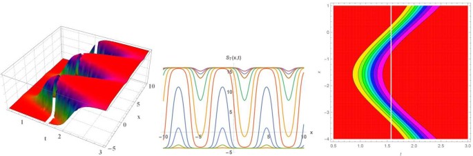

  

  Numerical simulations of Eq. (14) in three different types [$a_{0}=2$, $a_{2}=1$, $c=-3$, $\delta=-1$, $\mu=3$, $\sigma =5$, $\varrho=4$]

• Fig. 2 explains periodic solitary waves equations for Eq. (15) when [$a_{0}=2$, $a_{2}=1$, $c=-3$, $\delta=-1$, $\mu=3$, $\sigma=5$, $\varrho=4$].

  Figure 2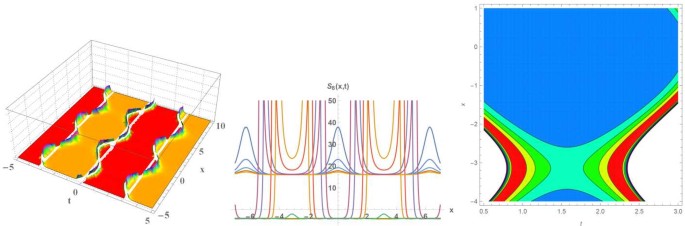

  

  Numerical simulations of Eq. (15) in three different types for [$a_{0}=2$, $a_{2}=1$, $c=-3$, $\delta=-1$, $\mu=3$, $\sigma=5$, $\varrho=4$]

• Fig. 3 explains periodic solitary waves equations for Eq. (17) when [$a_{0}=2$, $a_{2}=1$, $c=-3$, $\kappa=-1$, $\mu=3$, $\sigma=5$].

  Figure 3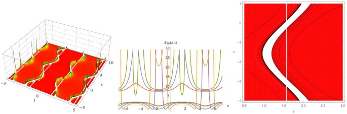

  

  Numerical simulations of Eq. (17) in three different types [$a_{0}=2$, $a_{2}=1$, $c=-3$, $\kappa=-1$, $\mu=3$, $\sigma =5$]

4 Stability

This section of our research paper investigates one of the basic properties of any model. It examines the stability property for the fractional nonlinear KS equation by using a Hamiltonian system. The momentum in the Hamiltonian system is given by the following formula:

$$\begin{aligned} M=\frac{1}{2} \int_{-\backepsilon}^{\backepsilon} \mathcal{S}^{2} (\wp)\, d\wp, \end{aligned}$$

(36)

where ϶ is an arbitrary constant. Thus, the condition for stability is given in the following condition:

$$\begin{aligned} \frac{\partial M}{\partial c} \bigg|_{c=\hslash}>0, \end{aligned}$$

(37)

where c, ℏ are arbitrary constants.

For an example of studying the stability of the solution of Eq. (3) by using (30) with the following values of the constants [$a_{0}=1$, $a_{2}=-1$, $\delta=-5$, $\mu=\frac{1}{25}$, $\sigma=\frac {1}{15}$, $\varrho=5$] yields

$$\begin{aligned} M={}& \frac{1}{15} \int_{-5} ^{5} \frac{1}{ (2 e^{50} \cosh (\frac{5 c}{t-\sqrt{\pi} t} )+e^{100}+1 )^{3}} \biggl[ 6 e^{50} \biggl(2 \bigl(e^{200}-1 \bigr)\sinh \biggl( \frac{5 c}{t-\sqrt{\pi} t} \biggr) \\ & +2 e^{50} \bigl(e^{100}-1 \bigr)\sinh \biggl(\frac{10 c}{t-\sqrt{\pi} t} \biggr)+75 \bigl(1+3 e^{100}+e^{200} \bigr) \cosh \biggl(\frac{5 c}{t-\sqrt{\pi} t} \biggr) \\ &+2 e^{50} \bigl(38+37 e^{100} \bigr) \cosh \biggl( \frac{10 c}{t-\sqrt{\pi} t} \biggr)+25 e^{100} \cosh \biggl(\frac{15 c}{t-\sqrt{\pi} t} \biggr) \biggr) \\&+74 e^{300}+684 e^{200}+666 e^{100}+76 \biggr] \,dt. \end{aligned}$$

(38)

Thus, we obtain

$$\begin{aligned} \frac{\partial M}{\partial c} \bigg|_{c=2}< 0. \end{aligned}$$

(39)

This means that this solution is unstable and, by applying the same steps to other obtained solutions, the stability property of each one of them can be determined.

5 Conclusion

This research has successfully applied the modified Khater method with a new fractional operator to the fractional nonlinear KS equation that is arising in the nonlinear wave processes in a liquid containing gas bubbles. This new operator is used to avoid the disadvantage of the other fractional operator. Distinct, solitary wave solutions have been obtained for this equation. For more illustrations of the dynamical behavior of this kind of fluid, some solutions have been sketched (Figs. 1, 2, 3) in three different formulas of each figure (two, three-dimensional, and contour plots).

References

Talaee, M., Shabibi, M., Gilani, A., Rezapour, S.: On the existence of solutions for a pointwise defined multi-singular integro-differential equation with integral boundary condition. Adv. Differ. Equ. 2020(1), Article ID 41 (2020)
Baleanu, D., Etemad, S., Pourrazi, S., Rezapour, S.: On the new fractional hybrid boundary value problems with three-point integral hybrid conditions. Adv. Differ. Equ. 2019(1), Article ID 473 (2019)
Baleanu, D., Ghafarnezhad, K., Rezapour, S., Shabibi, M.: On the existence of solutions of a three steps crisis integro-differential equation. Adv. Differ. Equ. 2018(1), Article ID 135 (2018)
Baleanu, D., Rezapour, S., Saberpour, Z.: On fractional integro-differential inclusions via the extended fractional Caputo–Fabrizio derivation. Bound. Value Probl. 2019(1), Article ID 79 (2019)
Aydogan, M.S., Baleanu, D., Mousalou, A., Rezapour, S.: On high order fractional integro-differential equations including the Caputo–Fabrizio derivative. Bound. Value Probl. 2018(1), Article ID 90 (2018)
Zhou, Q., Rezazadeh, H., Korkmaz, A., Eslami, M., Mirzazadeh, M., Rezazadeh, M.: New optical solitary waves for unstable Schrödinger equation in nonlinear medium. Opt. Appl. 49(1), 135–150 (2019)
Kumar, V.S., Rezazadeh, H., Eslami, M., Izadi, F., Osman, M.S.: Jacobi elliptic function expansion method for solving KdV equation with conformable derivative and dual-power law nonlinearity. Int. J. Appl. Comput. Math. 5(5), Article ID 127 (2019)
Baleanu, D., Jajarmi, A., Sajjadi, S.S., Mozyrska, D.: A new fractional model and optimal control of a tumor-immune surveillance with non-singular derivative operator. Chaos, Interdiscip. J. Nonlinear Sci. 29(8), Article ID 083127 (2019)
Jajarmi, A., Arshad, S., Baleanu, D.: A new fractional modelling and control strategy for the outbreak of dengue fever. Phys. A, Stat. Mech. Appl. 535, Article ID 122524 (2019)
Jajarmi, A., Ghanbari, B., Baleanu, D.: A new and efficient numerical method for the fractional modeling and optimal control of diabetes and tuberculosis co-existence. Chaos, Interdiscip. J. Nonlinear Sci. 29(9), Article ID 093111 (2019)
Baleanu, D., Sajjadi, S.S., Jajarmi, A., Asad, J.H.: New features of the fractional Euler–Lagrange equations for a physical system within non-singular derivative operator. Eur. Phys. J. Plus 134(4), Article ID 181 (2019)
Jajarmi, A., Baleanu, D., Sajjadi, S.S., Asad, J.H.: A new feature of the fractional Euler–Lagrange equations for a coupled oscillator using a nonsingular operator approach. Front. Phys. 7, Article ID 196 (2019)
Mohammadi, F., Moradi, L., Baleanu, D., Jajarmi, A.: A hybrid functions numerical scheme for fractional optimal control problems: application to nonanalytic dynamic systems. J. Vib. Control 24(21), 5030–5043 (2018)
Hajipour, M., Jajarmi, A., Baleanu, D.: On the accurate discretization of a highly nonlinear boundary value problem. Numer. Algorithms 79(3), 679–695 (2018)
Hajipour, M., Jajarmi, A., Malek, A., Baleanu, D.: Positivity-preserving sixth-order implicit finite difference weighted essentially non-oscillatory scheme for the nonlinear heat equation. Appl. Math. Comput. 325, 146–158 (2018)
Aydogan, S.M., Baleanu, D., Mousalou, A., Rezapour, S.: On approximate solutions for two higher-order Caputo–Fabrizio fractional integro-differential equations. Adv. Differ. Equ. 2017(1), Article ID 221 (2017)
Kojabad, E.A., Rezapour, S.: Approximate solutions of a sum-type fractional integro-differential equation by using Chebyshev and Legendre polynomials. Adv. Differ. Equ. 2017(1), Article ID 351 (2017)
Baleanu, D., Mousalou, A., Rezapour, S.: On the existence of solutions for some infinite coefficient-symmetric Caputo–Fabrizio fractional integro-differential equations. Bound. Value Probl. 2017(1), Article ID 145 (2017)
Baleanu, D., Mousalou, A., Rezapour, S.: A new method for investigating approximate solutions of some fractional integro-differential equations involving the Caputo–Fabrizio derivative. Adv. Differ. Equ. 2017(1), Article ID 51 (2017)
Baleanu, D., Rezapour, S., Mohammadi, H.: Some existence results on nonlinear fractional differential equations. Philos. Trans. R. Soc. A, Math. Phys. Eng. Sci. 371(1990), Article ID 20120144 (2013)
Agarwal, R.P., Baleanu, D., Hedayati, V., Rezapour, S.: Two fractional derivative inclusion problems via integral boundary condition. Appl. Math. Comput. 257, 205–212 (2015)
Alsaedi, A., Baleanu, D., Etemad, S., Rezapour, S.: On coupled systems of time-fractional differential problems by using a new fractional derivative. J. Funct. Spaces 2016, Article ID 4626940 (2016)
Mirhosseini-Alizamini, S.M., Rezazadeh, H., Eslami, M., Mirzazadeh, M., Korkmaz, A.: New extended direct algebraic method for the Tzitzica type evolution equations arising in nonlinear optics. Comput. Methods Differ. Equ. 8(1), 28–53 (2020)
Gao, W., Rezazadeh, H., Pinar, Z., Baskonus, H.M., Sarwar, S., Yel, G.: Novel explicit solutions for the nonlinear Zoomeron equation by using newly extended direct algebraic technique. Opt. Quantum Electron. 52(1), Article ID 52 (2020)
Liu, J.-G., Eslami, M., Rezazadeh, H., Mirzazadeh, M.: Rational solutions and lump solutions to a non-isospectral and generalized variable-coefficient Kadomtsev–Petviashvili equation. Nonlinear Dyn. 95(2), 1027–1033 (2019)
Khater, M.M., Lu, D., Attia, R.A.: Dispersive long wave of nonlinear fractional Wu–Zhang system via a modified auxiliary equation method. AIP Adv. 9(2), Article ID 025003 (2019)
Attia, R.A., Lu, D., Khater, M.M.A.: Chaos and relativistic energy-momentum of the nonlinear time fractional Duffing equation. Math. Comput. Appl. 24(1), Article ID 10 (2019)
Khater, M., Attia, R.A., Lu, D.: Explicit lump solitary wave of certain interesting \((3+ 1)\)-dimensional waves in physics via some recent traveling wave methods. Entropy 21(4), Article ID 397 (2019)
Khater, M., Attia, R., Lu, D.: Modified auxiliary equation method versus three nonlinear fractional biological models in present explicit wave solutions. Math. Comput. Appl. 24(1), Article ID 1 (2019)
Khater, M.M., Lu, D., Attia, R.A.: Erratum: “Dispersive long wave of nonlinear fractional Wu–Zhang system via a modified auxiliary equation method ” [AIP Adv. 9, 025003 (2019)]. AIP Adv. 9(4), Article ID 049902 (2019)
Li, J., Qiu, Y., Lu, D., Attia, R.A., Khater, M.: Study on the solitary wave solutions of the ionic currents on microtubules equation by using the modified Khater method. Therm. Sci. 23, S2053–S2062 (2019)
Rezazadeh, H., Korkmaz, A., Khater, M.M., Eslami, M., Lu, D., Attia, R.A.: New exact traveling wave solutions of biological population model via the extended rational sinh–cosh method and the modified Khater method. Mod. Phys. Lett. B 33(28), Article ID 1950338 (2019)
Alderremy, A.A., Attia, R.A., Alzaidi, J.F., Lu, D., Khater, M.: Analytical and semi-analytical wave solutions for longitudinal wave equation via modified auxiliary equation method and Adomian decomposition method. Therm. Sci. 23, S1943–S1957 (2019)
Ali, A.T., Khater, M.M., Attia, R.A., Abdel-Aty, A.-H., Lu, D.: Abundant numerical and analytical solutions of the generalized formula of Hirota–Satsuma coupled KdV system. Chaos Solitons Fractals 2019, Article ID 109473 (2019)
Khater, M.M., Lu, D., Attia, R.A.: Lump soliton wave solutions for the \((2+ 1)\)-dimensional Konopelchenko–Dubrovsky equation and KdV equation. Mod. Phys. Lett. B 33(18), Article ID 1950199 (2019)
Seadawy, A.R., Iqbal, M., Lu, D.: Nonlinear wave solutions of the Kudryashov–Sinelshchikov dynamical equation in mixtures liquid-gas bubbles under the consideration of heat transfer and viscosity. J. Taibah Univ. Sci. 13(1), 1060–1072 (2019)
Inc, M., Aliyu, A.I., Yusuf, A., Baleanu, D.: New solitary wave solutions and conservation laws to the Kudryashov–Sinelshchikov equation. Optik 142, 665–673 (2017)
Zhao, Y.-M.: F-expansion method and its application for finding new exact solutions to the Kudryashov–Sinelshchikov equation. J. Appl. Math. 2013, Article ID 895760 (2013)
Tu, J.-M., Tian, S.-F., Xu, M.-J., Zhang, T.-T.: On Lie symmetries, optimal systems and explicit solutions to the Kudryashov–Sinelshchikov equation. Appl. Math. Comput. 275, 345–352 (2016)
Ryabov, P.N.: Exact solutions of the Kudryashov–Sinelshchikov equation. Appl. Math. Comput. 217(7), 3585–3590 (2010)
Ayub, K., Khan, M.Y., Hassan, Q.M.U.: Some new exact solutions of a three-dimensional Kudryashov–Sinelshchikov equation in the bubbly liquid. J. Sci. Arts 17(1), 183–194 (2017)
Akram, G., Sadaf, M., Anum, N.: Solutions of time-fractional Kudryashov–Sinelshchikov equation arising in the pressure waves in the liquid with gas bubbles. Opt. Quantum Electron. 49(11), Article ID 373 (2017)
Gupta, A.K., Ray, S.S.: On the solitary wave solution of fractional Kudryashov–Sinelshchikov equation describing nonlinear wave processes in a liquid containing gas bubbles. Appl. Math. Comput. 298, 1–12 (2017)
Atangana, A., Koca, I.: Chaos in a simple nonlinear system with Atangana–Baleanu derivatives with fractional order. Chaos Solitons Fractals 89, 447–454 (2016)
Atangana, A., Gómez-Aguilar, J.F.: Numerical approximation of Riemann–Liouville definition of fractional derivative: from Riemann–Liouville to Atangana–Baleanu. Numer. Methods Partial Differ. Equ. 34(5), 1502–1523 (2018)
Khater, M.M.A., Baleanu, D.: On new analytical and semi-analytical wave solutions of the quadratic–cubic fractional nonlinear Schrödinger equation. Adv. Differ. Equ. (2019, submitted)
Khater, M.M.A., Baleanu, D.: On the new explicit computational and numerical solutions of the fractional nonlinear space–time Telegraph equation. Mod. Phys. Lett. A (2019, submitted)
Fernandez, A., Özarslan, M.A., Baleanu, D.: On fractional calculus with general analytic kernels. Appl. Math. Comput. 354, 248–265 (2019)
Algahtani, O.J.J.: Comparing the Atangana–Baleanu and Caputo–Fabrizio derivative with fractional order: Allen Cahn model. Chaos Solitons Fractals 89, 552–559 (2016)
Alkahtani, B.S.T.: Chua’s circuit model with Atangana–Baleanu derivative with fractional order. Chaos Solitons Fractals 89, 547–551 (2016)
Acknowledgements
Mostafa Khater would like to dedicate this paper to his mother, son (Adam), and the soul of his father. Their love, support, and constant care will never be forgotten.
Availability of data and materials
Not applicable.
Funding
China Scholarship Council (CSC) (20190832).
Author information
Authors and Affiliations
Contributions
All authors conceived of the study, participated in its design and coordination, drafted the manuscript, participated in the sequence alignment, and read and approved the final manuscript.
Corresponding author
Ethics declarations
Competing interests
The authors declare that they have no competing interests.
Additional information
Publisher’s Note
Springer Nature remains neutral with regard to jurisdictional claims in published maps and institutional affiliations.
Rights and permissions
Open Access This article is licensed under a Creative Commons Attribution 4.0 International License, which permits use, sharing, adaptation, distribution and reproduction in any medium or format, as long as you give appropriate credit to the original author(s) and the source, provide a link to the Creative Commons licence, and indicate if changes were made. The images or other third party material in this article are included in the article’s Creative Commons licence, unless indicated otherwise in a credit line to the material. If material is not included in the article’s Creative Commons licence and your intended use is not permitted by statutory regulation or exceeds the permitted use, you will need to obtain permission directly from the copyright holder. To view a copy of this licence, visit http://creativecommons.org/licenses/by/4.0/.
About this article
Cite this article
Yue, C., Khater, M.M.A., Attia, R.A.M. et al. The plethora of explicit solutions of the fractional KS equation through liquid–gas bubbles mix under the thermodynamic conditions via Atangana–Baleanu derivative operator. Adv Differ Equ 2020, 62 (2020). https://doi.org/10.1186/s13662-020-2540-3
Received:
Accepted:
Published:
DOI: https://doi.org/10.1186/s13662-020-2540-3