Dynamic properties of a discrete population model with diffusion

Abstract

We study the dynamical properties of a discrete population model with diffusion. We survey the transcritical, pitchfork, and flip bifurcations of nonhyperbolic fixed points by using the center manifold theorem. For the degenerate fixed point with eigenvalues ±1 of the model, we obtain the normal form of the mapping by using the coordinate transformation. Then we give an approximating system of the normal form via an approximation by a flow. We give the local behavior near a degenerate equilibrium of the vector field by the blowup technique. By the conjugacy between the reflection of time-one mapping of a vector field and the model we obtain the stability and qualitative structures near the degenerate fixed point of the model. Finally, we carry out a numerical simulation to illustrate the analytical results of the model.

1 Introduction

In recent years, discrete dynamic systems developed rapidly and achieved fruitful results (see [1–9]). Particularly, the dynamic properties of discrete population models received extensive attention by many researchers [10–15]. In [10] the authors considered the following discrete population model with diffusion:

$$ \mu _{i}^{t+1}=\frac{p \mu _{i}^{t}}{1+q \mu _{i}^{t}}+d \Delta ^{2} \mu _{i-1}^{t}, $$

(1)

with Dirichlet boundary condition $\mu _{0}^{t}=0=\mu _{n+1}^{t}$, where $d>0$ is the diffusion coefficient, $t \in Z^{+}=\{0,1,2, \ldots \}$, $p>1$, $q>0$, $\Delta ^{2}$ is second-order difference operator, and ${\Delta ^{2}}\mu _{i - 1}^{t} = \mu _{i + 1}^{t} - 2\mu _{i}^{t} + \mu _{i - 1}^{t}$, $i \in \{1,2, \ldots , n\}$.

When $n=2$, $p=q=b$, and $\mu _{1}^{t}$, $\mu _{2}^{t}$ are written as $\mu _{t}$, $\nu _{t}$, respectively, and model (1) can be transformed into a particular two-patch discrete-time metapopulation model of the form

$$ \textstyle\begin{cases} {\mu _{t+1}=\frac{b \mu _{t}}{1+b \mu _{t}}+d (-2 \mu _{t}+\nu _{t} )}, \\ {\nu _{t+1}=\frac{b \nu _{t}}{1+b \nu _{t}}+d (\mu _{t}-2 \nu _{t} )}.\end{cases} $$

(2)

The properties of pitchfork bifurcation, one case (i.e., $b=\frac{(d+1)^{2}}{3 d-1}$, $d>\frac{1}{3}$) of flip bifurcation at nontrivial fixed point $E_{1} (\mu ^{*}, \nu ^{*} )$ with $\mu ^{*}=\nu ^{*}=\frac{b-d-1}{b(d+1)}$, and Lyapunov exponential analysis are given in [10].

In this paper, we study the following problems. First, we focus on the stability and bifurcations of the nonhyperbolic fixed point $E_{0}(0,0)$ and on the case (i.e., $b=\frac{(d+1)^{2}}{d-1}$, $d>1$) of flip bifurcation at nontrivial fixed point $E_{1}$. Second, we investigate the stability and qualitative structures near a degenerate fixed point $\tilde{E}_{0}(0,0)$ formed by fixed points $E_{0}$ and $E_{1}$, which collide and bond together when $(d, b)=(1,2)$.

Compared to continuous models, discrete models can have different dynamic properties (see [1]), such as flip bifurcation (see [15]), Neimark–Sacker bifurcation (see [3, 14, 15]), invariant curve (see [15]), fold-flip bifurcation (see [8]), and strong resonance (see [3]).

The stability and qualitative structures near a degenerate fixed point of a discrete dynamic system are paid attention by many researchers; for example, Elaydi and Luís [7] proposed some open problems about stability of degenerate fixed point of discrete-time Guzowska–Luís–Elaydi competition model and discrete-time Ricker competition model. Due to the complexity of the degenerate fixed point, it is necessary to combine a variety of mathematical tools to study, for example, coordinate transformation [3], normal form theory (see [3, 16]), Picard iteration (see [3, 8]), approximation by a flow (see [3, 16]), qualitative theory of ordinary differential equations (see [17]), and blowup technique (see [17–19]). In this paper, we survey the local behavior near a degenerate equilibrium of a vector field by homogeneous polar blowup (see [18, 19]), which can avoid tedious calculations.

This paper is organized as follows. In Sect. 2, we give topological types of fixed point of model (2). In Sect. 3, we study transcritical bifurcation, pitchfork bifurcation, flip bifurcation, and the stability of the fixed point $E_{0}$ of model (2). In Sect. 4, a particular case ($b=\frac{(d+1)^{2}}{d-1}$, $d>1$) of flip bifurcation and stability of fixed point $E_{1}$ of model (2) are surveyed. In Sect. 5, we apply the coordinate transformation to obtain the normal form of the mapping of model (2) near the degenerate fixed point $\tilde{E}_{0}$. The approximate system (also called a vector field) of the normal form of the mapping is given by Takens’s theorem (see [16, pp. 142–148]) and Picard iteration. The local behavior near the degenerate equilibrium $(0,0)$ of the vector field is obtained by using the blowup technique. The stability and qualitative structures near the degenerate fixed point $\tilde{E}_{0}$ of model (2) are obtained by the conjugacy between reflection of time-one mapping of the vector field and model (2). Finally, we perform numerical simulation analysis.

2 Topological types of the fixed point

In this section, we give topological types of fixed points $E_{0}$ and $E_{1}$ on the parameter $(d,b)$-plane. We write model (2) as the following planar mapping $T : \mathbb{R}^{2} \mapsto \mathbb{R}^{2}$:

$$ T : \begin{pmatrix} {\mu } \\ {\nu }\end{pmatrix} \mapsto \begin{pmatrix} {\frac{b \mu }{1+b \mu }+d(-2 \mu +v)} \\ {\frac{b \nu }{1+b \nu }+d(\mu -2 v)}\end{pmatrix}. $$

The mapping T expanded by Taylor series at the fixed point $E_{0}$ is

$$ \begin{pmatrix} {\mu } \\ {\nu }\end{pmatrix} \mapsto \begin{pmatrix} {b-2 d} & {d} \\ {d} & {b-2 d}\end{pmatrix} \begin{pmatrix} {\mu } \\ {\nu }\end{pmatrix}+ \begin{pmatrix} {-b^{2} \mu ^{2}+b^{3} \mu ^{3}} \\ {-b^{2} \nu ^{2}+b^{3} \nu ^{3}}\end{pmatrix}+O(3), $$

(3)

where $O(3)$ represents the terms of orders greater than or equal to 3. The Jacobian matrix of T at the point ${E}_{0}$ is

$$ J (E_{0} )= \begin{pmatrix} {b-2 d} & {d} \\ {d} & {b-2 d}\end{pmatrix}. $$

The eigenvalues of matrix $J (E_{0} )$ are $\lambda _{1}=b-d$ and $\lambda _{2}=b-3 d$.

Translating the fixed point $E_{1}$ into the origin O by coordinate translation $y_{1}=\mu -\mu ^{*}$, $y_{2}=\nu -\nu ^{*}$, the Taylor expansion at the fixed point $E_{1}$ is

$$ \tilde{T}: \begin{pmatrix} {y_{1}} \\ {y_{2}}\end{pmatrix} \mapsto \begin{pmatrix} {\frac{(d+1)^{2}}{b}-2 d} & {d} \\ {d} & {\frac{(d+1)^{2}}{b}-2 d}\end{pmatrix} \begin{pmatrix} {y_{1}} \\ {y_{2}}\end{pmatrix}+ \begin{pmatrix} {-\frac{(d+1)^{3}}{b} y_{1}^{2}+\frac{(d+1)^{4}}{b} y_{1}^{3}} \\ {-\frac{(d+1)^{3}}{b} y_{2}^{2}+\frac{(d+1)^{4}}{b} y_{2}^{3}}\end{pmatrix}+O(3). $$

(4)

The Jacobian matrix of T at the fixed point $E_{1}$ (i.e., mapping T̃ at the fixed point O) is as follows:

$$ J ({E}_{1} )= \begin{pmatrix} {\frac{(d+1)^{2}}{b}-2 d} & {d} \\ {d} & {\frac{(d+1)^{2}}{b}-2 d}\end{pmatrix}. $$

The eigenvalues of matrix $J (E_{1} )$ are $\lambda _{3}=\frac{(d+1)^{2}}{b}-d$ and $\lambda _{4}=\frac{(d+1)^{2}}{b}-3 d$.

For convenience, we give some notations: $D_{i}$ ($i=1,2,\ldots ,6$) (see Fig. 1), and $\aleph _{i}$ ($i=1,2,\ldots ,12$) (see Fig. 2) are the regions of the parameter $(d,b)$-plane of $E_{0}$ and $E_{1}$, respectively, divided by the curves $\beta _{i}$ ($i=1,2,3,4$) and $\gamma _{i}$ ($i=1,2,\ldots ,6$):

$$\begin{aligned} &{{\beta _{1}} \stackrel{{{\Delta }}}{=} \bigl\{ {(d,b) \in {\mathbb{R}^{2}}|b = d + 1,d > 0} \bigr\} , \qquad {\beta _{2}} \stackrel{{{\Delta }}}{=} \bigl\{ {(d,b) \in { \mathbb{R}^{2}}|b = d - 1,d > 1} \bigr\} ,} \\ &{{\beta _{3}} \stackrel{{{\Delta }}}{=} \bigl\{ {(d,b) \in { \mathbb{R}^{2}}|b = 3d + 1,d > 0} \bigr\} ,\qquad {\beta _{4}} \stackrel{{{\Delta }}}{=} \biggl\{ {(d,b) \in {\mathbb{R}^{2}}\Big|b = 3d - 1,d > \frac{1}{3}} \biggr\} ,} \\ &{\gamma _{1}} \stackrel{{{\Delta }}}{=} \biggl\{ {(d,b) \in { \mathbb{R}^{2}}\Big|b = \frac{{{{(d + 1)}^{2}}}}{{d - 1}},d > 1,b > 0} \biggr\} ,\qquad { \gamma _{2}} \stackrel{{{\Delta }}}{=} {\beta _{1}}, \\ & { \gamma _{3}} \stackrel{{{\Delta }}}{=} \biggl\{ {(d,b) \in { \mathbb{R}^{2}}\Big|b = \frac{{{{(d + 1)}^{2}}}}{{3d - 1}},d > \frac{1}{3},b > 0} \biggr\} , \\ &{\gamma _{4}} \stackrel{{{\Delta }}}{=} \biggl\{ {(d,b) \in { \mathbb{R}^{2}}\Big|b = \frac{{{{(d + 1)}^{2}}}}{{3d + 1}},d > 0} \biggr\} ,\qquad {\gamma _{5}} \stackrel{{{\Delta }}}{=} \bigl\{ {(d,b) \in {\mathbb{R}^{2}}|b = 1,d > 0} \bigr\} , \\ &{\gamma _{6}} \stackrel{{{ \Delta }}}{=} \biggl\{ {(d,b) \in {\mathbb{R}^{2}}\Big|b = \frac{1}{3},d > 0} \biggr\} . \end{aligned}$$

Figure 1

Regions in the parameter $(d,b)$-plane of $E_{0}$

Figure 2

Regions in the parameter $(d,b)$-plane of $E_{1}$

Lemma 1

The fixed point $E_{0}$ is nonhyperbolic if and only if $(d,b)$ lies on the curves $\beta _{i}$ ($i=1,2,3,4$). Otherwise, the fixed point $E_{0}$ has the following properties:

• (1) If $(d, b) \in D_{i}$ ($i=3$), then it is a stable node;

• (2) If $(d, b) \in D_{i}$ ($i=1,5,6$), then it is an unstable node;

• (3) If $(d, b) \in D_{i}$ ($i=2,4$), then it is a saddle.

Lemma 2

The fixed point $E_{1}$ is nonhyperbolic if and only if $(d, b)$ lies on the curves $\gamma _{i}$ ($i=1,2,3,4,5,6$). Otherwise, the fixed point $E_{1}$ has the following properties:

• (1) If $(d, b)\in \aleph _{i}$ ($i=8,12$), then it is a stable node;

• (2) If $(d, b)\in \aleph _{i}$ ($i=1,3,5,6,10$), then it is a unstable node;

• (3) If $(d, b)\in \aleph _{i}$ ($i=2,4,7,9,11$), then it is a saddle.

3 Bifurcation at fixed point $E_{0}$

In this section, the parameter b is regarded as a bifurcation parameter. We survey stability and bifurcation properties of the mapping T at the fixed point $E_{0}$.

Theorem 1

As $(d, b)$ passes through the curve $\beta _{1}$, the mapping T undergoes a transcritical bifurcation at the fixed point $E_{0}$. The details are as follows:

• (1) The fixed points $E_{0}$ and $E_{1}$ collide and bond together to form a fixed point when $(d, b)$ passes through curve $\beta _{1}$;

• (2) The fixed point $E_{0}$ is nonhyperbolic and stable for $0< d<1$ when $(d, b)$ lies on the curve $\beta _{1}$;

• (3) The fixed point $E_{0}$ is nonhyperbolic and unstable for $d>1$ when $(d, b)$ lies on the curve $\beta _{1}$.

Proof

Mapping (3) can be diagonalized by the linear transformation $\mu =x+y$, $\nu =x-y$ when $b=d+1$. We obtain the following mapping:

$$ \begin{pmatrix} {x} \\ {y} \\ {b}\end{pmatrix} \mapsto \begin{pmatrix} {\lambda _{1}} & {0} & {0} \\ {0} & {\lambda _{2}} & {0} \\ {0} & {0} & {1}\end{pmatrix} \begin{pmatrix} {x} \\ {y} \\ {b}\end{pmatrix}+ \begin{pmatrix} {-b^{2} (x^{2}+y^{2} )+b^{3} (x^{3}+3 x y^{2} )} \\ {-2 b^{2} x y+b^{3} (y^{3}+3 x^{2} y )} \\ {0}\end{pmatrix}+O(3). $$

(5)

We choose b as a bifurcation parameter. According to the center manifold theorem [20], a center manifold of mapping (5) is

$$ W^{c}= \bigl\{ (x, y, b)|y=h(x, b), h (0, b_{0} )=D h (0, b_{0} )=0, \vert x \vert < \varepsilon , \vert b-b_{0} \vert < \delta \bigr\} , $$

where $b_{0} :=d+1$, and ε and δ are sufficiently small positives. Therefore assume that the center manifold form is

$$ y=h_{1}(x, b)=d_{1} x^{2}+e_{1} (b-b_{0} ) x+f_{1} (b-b_{0} )^{2}+O(3), $$

which must satisfy

$$ \begin{aligned} &h_{1} \bigl(\lambda _{1} x-b^{2} \bigl(x^{2}+h_{1}^{2}(x, b) \bigr)+b^{3} \bigl(x^{3}+3 x h_{1}^{2}(x, b) \bigr)+O(3), b \bigr) \\ &\quad =\lambda _{2} h_{1}(x, b)-2 b^{2} x h_{1}(x, b)+b^{3} \bigl(h_{1}^{3}(x, b)+3 x^{2}(x, b) \bigr). \end{aligned} $$

By comparing the coefficients we obtain $d_{1}=\lambda _{2} d_{1}$, $e_{1}=\lambda _{2} e_{1}$, $f_{1}=\lambda _{2} f_{1}$. We havee $\lambda _{1}=1$ and $\lambda _{2}=1-2 d$ when $(d, b)$ lies on the curve $\beta _{1}$. Therefore $d_{1}=e_{1}=f_{1}=0$. The center manifold is

$$ y=h_{1}(x, b)=O(3). $$

By substituting the center manifold $y=h_{1}(x, b)$ into mapping (5) we obtain a one-dimensional mapping reduced to the center manifold as follows:

$$ x \mapsto f_{1}(x)=x-b^{2} x^{2}+b^{3} x^{3}+O(3). $$

We can verify that the transversality and nondegeneracy conditions of transcritical bifurcation (see [4, pp. 504–507])

$$ \frac{\partial f_{1}}{\partial x}\bigg|_{(x, b)= (0, b_{0} )}=1,\qquad \frac{\partial ^{2} f_{1}}{\partial x \partial b} \bigg|_{(x, b)= (0, b_{0} )}=1 \neq 0,\qquad \frac{\partial ^{2} f_{1}}{\partial x^{2}}\bigg|_{(x, b)= (0, b_{0} )}=-2 b^{2} \neq 0 $$

are established. Therefore the mapping T undergoes a transcritical bifurcation at the fixed point $E_{0}$ as $(d, b)$ passes through the curve $\beta _{1}$. We obtain by Theorem 1.15 in [5, p. 29] and $\lambda _{1}=1$, $\lambda _{2}=1-2 d \neq 1$ that the fixed point $E_{0}$ is stable and nonhyperbolic for $0< d<1$ when $(d, b)$ lies on the curve $\beta _{1}$. The fixed point $E_{0}$ is unstable and nonhyperbolic for $d>1$ when $(d, b)$ lies on the curve $\beta _{1}$. The proof of the theorem is completed. □

Remark 1

The mapping

$$ x \mapsto f_{1}(x)=x-b^{2} x^{2}+b^{3} x^{3}+O(3) $$

can be seen as

$$ x \mapsto f_{1}(x)=(b-d)x-b^{2} x^{2}+b^{3} x^{3}+O(3) $$

when $(b,d)$ lies on $\beta _{1}$. Therefore

$$ \frac{\partial ^{2} f_{1}}{\partial x \partial b}\bigg|_{(x, b)= (0, b_{0} )}=1. $$

Theorem 2

As $(d, b)$ passes through the curve $\beta _{2}$, the mapping T undergoes a flip bifurcation at fixed point $E_{0}$. The details are as follows:

• (1) The mapping T appears in a stable 2-period orbit near fixed point $E_{0}$, and the stability of fixed point does not change when $(d, b)$ passes through the curve $\beta _{2}$;

• (2) The fixed point $E_{0}$ is nonhyperbolic and unstable when $(d, b)$ lies on the curve $\beta _{2}$.

Proof

Similarly, the center manifold has the form

$$ y = {h_{2}}(x,b) = {d_{2}} {x^{2}} + {e_{2}}(b -{b_{1}})x + {f_{2}} {(b-{b_{1}})^{2}} + O(3) $$

when $b=b_{1} :=d-1$. The center manifold

$$ y = {h_{2}}(x,b) = O(3) $$

can be obtained by the same calculation method as in Theorem 1. By substituting the center manifold into mapping (5) we obtain the following one-dimensional mapping reduced to the center manifold:

$$ x \mapsto {f_{2}}(x) = - x - {b^{2}} {x^{2}} + {b^{3}} {x^{3}} + O(3). $$

We can verify that the transversality and nondegeneracy conditions of flip bifurcation (see Theorem 4.3 in [3])

$$\begin{aligned}& {F_{1}} { {: = \frac{{{\partial ^{2}}{f_{2}}}}{{\partial x\partial b}}} \bigg|_{(x,b) = (0,{b_{1}})}} = - 1, \\& {{F_{2}}: = \biggl[ {\frac{1}{2}{{ \biggl( { \frac{{{\partial ^{2}}{f_{2}}}}{{\partial {x^{2}}}}} \biggr)}^{2}} + \frac{1}{3} \biggl( { \frac{{{\partial ^{3}}{f_{2}}}}{{\partial {x^{3}}}}} \biggr)} \biggr]} \bigg|_{(x,b) = (0,{b_{1}})} = 2{b^{3}}(b + 1) > 0 \end{aligned}$$

are established. Note that the mapping T undergoes a flip bifurcation as $(d, b)$ passes through the curve $\beta _{2}$. By Theorem 3.5.1 in [6] and $F_{2}>0$ the mapping T appears in a stable 2-period orbit as $(d, b)$ passes through the curve $\beta _{2}$. We have ${\lambda _{1}} = - 1$ and ${\lambda _{2}} < - 1$ when $(d, b)$ lies on the curve $\beta _{2}$. So the nonhyperbolic fixed point $E_{0}$ is unstable. The proof of the theorem is completed. □

Theorem 3

As $(d, b)$ passes through the curve $\beta _{3}$, the mapping T undergoes a pitchfork bifurcation at the fixed point $E_{0}$. The details are as follows:

• (1) The stability of the fixed point $E_{0}$ does not change when $(d, b)$ passes through the curve $\beta _{3}$;

• (2) The fixed point $E_{0}$ is nonhyperbolic and unstable when $(d, b)$ lies on the curve $\beta _{3}$.

Proof

Applying the same calculation method as in Theorem 1, we obtain the center manifold

$$ x = {h_{3}}(y,b) = \frac{{{b^{2}}}}{{2d}}{y^{2}} + O(3) $$

when $b = {b_{2}}: = 3d + 1$. Substituting the center manifold $x = {h_{3}}(y,b)$ into mapping (2) yields a one-dimensional mapping reduced to the center manifold

$$ y \mapsto {f_{3}}(y) = y - \frac{{{b^{4}}}}{d}{y^{3}} + O(3). $$

We can check that the transversality and nondegeneracy conditions of pitchfork bifurcation (see [4, p. 511])

$$\begin{aligned}& { {\frac{{\partial {f_{3}}}}{{\partial y}}} \bigg|_{(y,b) = (0,{b_{2}})}} = 1,\qquad { { \frac{{{\partial ^{2}}{f_{3}}}}{{\partial y\partial b}}} \bigg|_{(y,b) = (0,{b_{2}})}} = 1, \\& { {\frac{{{\partial ^{2}}{f_{3}}}}{{\partial {y^{2}}}}} \bigg|_{(y,b) = (0,{b_{2}})}} = 0,\qquad { { \frac{{{\partial ^{3}}{f_{3}}}}{{\partial {y^{3}}}}} \bigg|_{(y,b) = (0,{b_{2}})}} = \frac{{18{b^{3}}(b + 1)}}{{1 - b}} \end{aligned}$$

are established. Therefore the mapping T undergoes a pitchfork bifurcation at fixed point $E_{0}$ as $(d, b)$ passes through the curve $\beta _{3}$. We have ${\lambda _{1}}=3d + 1 > 1$ and ${\lambda _{2}}=1$ when $(d, b)$ lies on the curve $\beta _{3}$. Therefore the fixed point $E_{0}$ is nonhyperbolic and stable when $(d, b)$ lies on the curve $\beta _{3}$. The proof of the theorem is completed. □

Theorem 4

As $(d, b)$ passes through the curve $\beta _{4}$, the mapping T undergoes a flip bifurcation at fixed point $E_{0}$. The details are as follows:

• (1) For $d \in (\frac{1}{3},1)$, the mapping T appears in a stable 2-periodic orbit near fixed point $E_{0}$, and the stability of fixed point $E_{0}$ has to change when $(d, b)$ passes through the curve $\beta _{4}$;

• (2) For $d \in (1, + \infty )$, the mapping T appears in a repellent 2-period orbit near fixed point $E_{0}$, and the stability of fixed point $E_{0}$ does not change when $(d, b)$ passes through the curve $\beta _{4}$;

• (3) The fixed point $E_{0}$ is stable and nonhyperbolic for $d \in (\frac{1}{3},1)$ when $(d, b)$ lies on the curve $\beta _{4}$;

• (4) The fixed point $E_{0}$ is unstable and nonhyperbolic for $d \in (1, + \infty )$ when $(d, b)$ lies on the curve $\beta _{4}$.

Proof

Similarly, when $b = {b_{3}}: = 3d - 1$, we obtain the center manifold as follows:

$$ x = {h_{4}}(y,b) = \frac{{{b^{2}}}}{{2(d - 1)}}{y^{2}} + O(3). $$

Substituting the center manifold $x = {h_{4}}(y,b)$ into mapping (5), we obtain a one-dimensional mapping reduced to the center manifold,

$$ y \mapsto {f_{4}}(y) = - y - \frac{{{b^{4}}}}{{d - 1}}{y^{3}} + O(3). $$

We can check that the transversality and nondegeneracy conditions of flip bifurcation

$$ {F_{3}}:= \frac{{{\partial ^{2}}{f_{4}}}}{{\partial y\partial b}} \bigg|_{{ (y,b) = (0,{b_{3}})}} = - 1,\qquad {{F_{4}}: = \biggl[ { \frac{1}{2}{{ \biggl( { \frac{{{\partial ^{2}}{f_{4}}}}{{\partial {y^{2}}}}} \biggr)}^{2}} + \frac{1}{3} \biggl( { \frac{{{\partial ^{3}}{f_{4}}}}{{\partial {y^{3}}}}} \biggr)} \biggr]} \bigg|_{{(y,b) = (0,{b_{3}})}} = \frac{{2{b^{4}}}}{{1 - d}} $$

are established. The mapping T undergoes a flip bifurcation as $(d, b)$ passes through the curve $\beta _{4}$ at fixed point $E_{0}$. By Theorem 3.5.1 in [6] the mapping T appears in a stable 2-periodic orbit for $d \in (\frac{1}{3},1)$ and in a repellent 2-periodic orbit for $d \in (1, + \infty )$. We have ${\lambda _{1}} = 2d - 1$ and ${\lambda _{2}} = - 1$ when $(d,b)$ lies on the curve $\beta _{4}$. By Theorem 1.61 in [5] the fixed point $E_{0}$ is unstable and nonhyperbolic for $d \in (1, + \infty )$ and stable and nonhyperbolic for $d \in (\frac{1}{3},1)$. The proof of the theorem is completed. □

4 Bifurcation at fixed point $E_{1}$

In this section, we consider b as a bifurcation parameter and apply the center manifold theorem to survey the stability and flip bifurcation of the fixed point $E_{1}$ of the mapping T.

Theorem 5

As $(d, b)$ passes through the curve $\gamma _{1}$, the mapping T undergoes a flip bifurcation at fixed point $E_{1}$. The details are as follows:

• (1) The mapping T appears in a stable 2-periodic orbit near fixed point $E_{1}$, and the stability of the fixed point $E_{1}$ does not change when $(d, b)$ passes through the curve $\gamma _{1}$;

• (2) The fixed point $E_{1}$ is nonhyperbolic and unstable when $(d, b)$ lies on the curve $\gamma _{1}$.

Proof

The mapping T̃ can be diagonalized into the following form by linear transformation $y_{1} = x + y$, $y_{2} = x - y$ when $b = {b_{4}}: = \frac{{{{(d + 1)}^{2}}}}{{d - 1}}$ ($d>1$):

$$\left(\begin{array}{c}x\\ y\\ b\end{array}\right)\mapsto \left(\begin{array}{ccc}{\lambda }_3& 0& 0\\ 0& {\lambda }_4& 0\\ 0& 0& 1\end{array}\right)\left(\begin{array}{c}x\\ y\\ b\end{array}\right)+\left(\begin{array}{c}-\frac{2{(d+1)}^2}{b}(x^2+y^2)+\frac{6{(d+1)}^4}{b}(x^3+3x{y}^2)\\ -\frac{4{(d+1)}^3}{b}xy+\frac{6{(d+1)}^4}{b}(y^3+3x^{2}y)\\ 0\end{array}\right)+O(3).$$

(6)

Similarly to the previous proof method, we get that the center manifold of mapping (6) is

$$ y = {h_{5}}(x,b) = O(3). $$

Substituting the center manifold into mapping (6), we obtain the one-dimensional mapping reduced to the center manifold

$$ x \mapsto {f_{5}}(x) = - x - (d - 1) (d + 1){x^{2}} + (d - 1){(d + 1)^{2}} {x^{3}} + O(3). $$

We can verify that the transversality and nondegeneracy conditions of flip bifurcation

$$\begin{aligned}& {F_{5}} : = \frac{{{\partial ^{2}}{f_{5}}}}{{\partial x\partial b}} \bigg|_{(x,b) = (0,{b_{4}})} = - 1, \\& {{F_{6}}: = \biggl[ {\frac{1}{2}{{ \biggl( { \frac{{{\partial ^{2}}{f_{5}}}}{{\partial {x^{2}}}}} \biggr)}^{2}} + \frac{1}{3} \biggl( { \frac{{{\partial ^{3}}{f_{5}}}}{{\partial {x^{3}}}}} \biggr)} \biggr]} \bigg|_{(x,b) = (0,{b_{4}})} = 2d(d - 1){(d + 1)^{2}} \end{aligned}$$

are established. The mapping T̃ undergoes a flip bifurcation as $(d, b)$ passes through the curve $\gamma _{1}$ at fixed point $E_{1}$. By Theorem 3.5.1 in [6] and $F_{6}>0$ mapping (4) appears in a stable 2-period orbit near fixed point $E_{1}$ for $d \in (1, + \infty )$ as $(d, b)$ passes through the curve $\gamma _{1}$. We have ${\lambda _{1}} = 2d - 1>1$ and ${\lambda _{2}} = - 1$ when $(d, b)$ lies on the curve $\gamma _{1}$, so the fixed point $E_{1}$ is nonhyperbolic and unstable. The proof of the theorem is completed. □

5 Qualitative structures and stability of degenerate fixed point

In this section, we apply Picard iteration, approximation by a flow, and near identity transformation (see [3, 8, 16]) to investigate the degenerate fixed point of the mapping T when $(d, b)=(1,2)$. We obtain qualitative structures and the stability of the degenerate fixed point of model (2).

5.1 Normal form

To establish the normal form of the mapping T, we write it in the following form when $(d, b)=(1,2)$:

$$ x \mapsto f(x) = Ax + R(x),\quad x=(\mu ,\nu )^{T}\in \mathbb{R}^{2}. $$

(7)

The matrix A has the eigenvalues ${\lambda _{1}} = 1$ and ${\lambda _{2}} = - 1$. From

$$ A{q_{1}} = {\lambda _{1}} {q_{1}},\qquad A{q_{2}} = {\lambda _{2}} {q_{2}},\qquad {A^{T}} {p_{1}} = {\lambda _{1}} {p_{1}},\qquad {A^{T}} {p_{2}} = {\lambda _{2}} {p_{2}} $$

we get the solution

$$ {p_{1}} = {q_{1}} = { \biggl(\frac{1}{{\sqrt{2} }}, \frac{1}{{\sqrt{2} }} \biggr)^{T}},\qquad {p_{2}} = {q_{2}} = { \biggl(\frac{1}{{\sqrt{2} }}, - \frac{1}{{\sqrt{2} }} \biggr)^{T}}. $$

Apply the reversible linear transformation

$$ \Phi _{1} :x = {\xi _{1}} {q_{1}} + {\xi _{2}} {q_{2}} $$

to mapping (7). Since $\langle {q_{1}},{p_{2}}\rangle = \langle {q_{2}},{p_{1}}\rangle = 0$, the linear transformation $\Phi _{1}$ transforms mapping (7) into the mapping

$$F:\left(\begin{array}{c}{\xi }_1\\ {\xi }_2\end{array}\right)\mapsto \left(\begin{array}{c}{\lambda }_1{\xi }_1+{\sum }_{i+j=2,3}\frac{1}{i!j!}{g}_{ij}{\xi }_1^i{\xi }_2^j\\ {\lambda }_2{\xi }_2+{\sum }_{i+j=2,3}\frac{1}{i!j!}{h}_{ij}{\xi }_1^i{\xi }_2^j\end{array}\right)+O\left({\parallel \xi \parallel }^4\right),$$

where

$$ \begin{aligned} &{g_{20}} = {g_{02}} = - 4 \sqrt{2} ,\qquad {g_{11}} = {g_{21}} = {g_{03}} = 0,\qquad {g_{30}} = {g_{12}} = 24, \\ &{h_{11}} = - 4\sqrt{2} ,\qquad {h_{20}} = {h_{02}} = {h_{30}} = {h_{12}} = 0,\qquad {h_{21}} = {h_{03}} = 24. \end{aligned} $$

Theorem 6

The smooth mapping F can be transformed into the following normal form by reversible near identity transformation:

$$\tilde{F}:\left(\begin{array}{c}{\eta }_1\\ {\eta }_2\end{array}\right)\mapsto \left(\begin{array}{c}{\eta }_1+a_0{\eta }_1^2+b_0{\eta }_2^2+c_0{\eta }_1^3+d_0{\eta }_1{\eta }_2^2\\ -{\eta }_1+{\eta }_1{\eta }_2\end{array}\right)+O\left({\parallel \eta \parallel }^4\right),$$

(8)

where

$$ {a_{0}} = \frac{1}{2},\qquad {b_{0}} = 16,\qquad {c_{0}} = \frac{1}{8},\qquad {d_{0}} = 12. $$

Proof

First, we apply the near identity transformation

$$ \Phi _{2} :{\xi _{1}} = {\eta _{1}} - \frac{{{h_{21}}}}{{2{h_{11}}}} \eta _{1}^{2} - \frac{{{h_{03}}}}{{6{h_{11}}}}\eta _{2}^{2},\qquad {\xi _{2}} = {\eta _{2}} $$

and scale transformation

$$ {\eta _{1}} \mapsto \frac{{{\eta _{1}}}}{{{h_{11}}}} $$

to mapping F to eliminate quadratic and cubic items as much as possible. Then the resonance term is left, and the normal form is obtained. The proof is complete. □

5.2 Approximation by a flow

For dealing with stability and qualitative structures near the degenerate fixed points of a planar mapping with eigenvalues ±1, the general idea is embedding the reflection of the normal form of a mapping into the flow of a vector field. Then we study the dynamic behavior of the mapping by the properties of the vector field. In [3, p. 424], it is stated that “any mapping sufficiently close to the identity mapping can be approximated up to any order by a flow shift.” That is, an approximating system (see [3]) can be constructed, in which the unit time shift ${\varphi ^{1}}$ along orbits coincides with (or, at least, approximates) the near identity mapping up to order k. In this paper, we use the reflection transformation (see [3, 8]) to transform the truncated normal form of the mapping F̃ into a near identity mapping and embed it into the flow of a vector field. We use the vector field to investigate the stability and qualitative structures near the degenerate fixed point of the mapping T when $(d, b)=(1,2)$. The Taken theorem and the following lemma come from [21, p. 38].

Lemma 3

(Taken’s)

Let $F:\mathbb{R}^{n}\rightarrow \mathbb{R}^{n}$ be the $C^{r}$-diffeomorphism ($r\geq 2$) defined by

$$ F ( x ) = Ax + {F^{2}} ( x ) + {F^{3}} ( x ) + \cdots + {F^{r}} ( x ) + o \bigl( {{{ \vert x \vert }^{r}}} \bigr)\quad \textit{as } x \to 0, $$

where $A = S(I + N)$, S is semisimple, N is nilpotent, $SN = NS$, and I is the identity. Let $1 < l < r$ be any integer, and let $F^{k}\in H_{n}^{k}$, where $H_{n}^{k}$ is the vector space of homogeneous polynomials of order k in n variables with values in $C^{n}$. Then there exist a diffeomorphism $\psi _{l}:\Omega \subseteq \mathbb{R}^{n}\rightarrow \mathbb{R}^{n}$, where Ω is a neighborhood of the origin in $\mathbb{R}^{n}$, and a vector field $X(x)$ on $\mathbb{R}^{n}$ such that

• (i) ${\verb"j"^{l}}({\psi _{l}} \circ F \circ \psi _{l}^{ - 1})$ is an A-normal form of diffeomorphism $F(x)$ up to order l,

• (ii) $X(Sx) = SX(x)$ for all $x\in \mathbb{R}^{n}$,

• (iii) ${\verb"j"^{l}}({\psi _{l}} \circ F \circ \psi _{l}^{ - 1})(x) = { \verb"j"^{l}}({\Phi _{X}}(1,Sx))$,

where $\verb"j"^{l}$ is the truncation operator up to order l, and ${\Phi _{X}}(t,x)$ is the flow of $X(x)$. Furthermore, for such a vector field $X(x)$, $\verb"j"^{l}X(x)$ is uniquely determined by $\verb"j"^{l}F(x)$.

If there exist constants k, σ, η such that

$$ \bigl\Vert Y(x,y) \bigr\Vert \geq \sigma \bigl\Vert (x,y) \bigr\Vert ^{k},\quad (x,y)\in \mathbb{R}^{2}, \bigl\Vert (x,y) \bigr\Vert \leq \eta , $$

then the $C^{\infty }$ vector field is of Łojasiewicz type, where $\|\cdot \|$ is the Euclidean norm on $\mathbb{R}^{2}$.

Lemma 4

Let $g\in \operatorname{Diff}(2)$ with associated formal normal form $\tilde{G} = R\circ \tilde{X_{1}}$ ($X \mapsto X_{1}$, i.e., time-one mapping), where X̃ has in 0 a singularity of Łojasiewicz type with a characteristic orbit and $R^{n} = I$ for some $n > 0$. Suppose, moreover, that all singularities in some nice decomposition of X̃ are of type I and, restricted to a fundamental conic domain ∑, we have $\alpha (g^{n}|\sum )\in [\operatorname{Diff}^{0}_{\mathrm{rot}}(2)]^{k}$ (this especially is the case where X̃ has no elliptic sectors). Then there exists a $C^{\infty }$-coordinate change H with $\verb"j"_{\infty }(H-I)(0)=0$ and an R-invariant representative X of X̃ such that $H^{-1}\circ g \circ H= R\circ \tilde{X}_{1}$.

Remark 2

Lemmas 3 and 4 deal with many concepts, the details of which can be found in [16] and [21], respectively.

For the truncated normal form of the mapping F̃,

$$N:\left(\begin{array}{c}{\eta }_1\\ {\eta }_2\end{array}\right)\mapsto \left(\begin{array}{c}{\eta }_1+a_0{\eta }_1^2+b_0{\eta }_2^2+c_0{\eta }_1^3+d_0{\eta }_1{\eta }_2^2\\ -{\eta }_1+{\eta }_1{\eta }_2\end{array}\right),$$

(9)

we can see that

$$R\circ N:\left(\begin{array}{c}{\eta }_1\\ {\eta }_2\end{array}\right)\mapsto \left(\begin{array}{c}{\eta }_1+a_0{\eta }_1^2+b_0{\eta }_2^2+c_0{\eta }_1^3+d_0{\eta }_1{\eta }_2^2\\ {\eta }_1-{\eta }_1{\eta }_2\end{array}\right)$$

and $RN(x) = N(Rx)$. For $R \circ N$ embedded in the flow of a vector field, we have the following results.

Theorem 7

The mapping $R \circ N$ satisfies

$$ R \circ N(\eta ) = {\varphi ^{t}}(\eta ) + O \bigl({ \Vert \eta \Vert ^{4}} \bigr) $$

in a small neighborhood of the origin O, where $\varphi ^{t}$ is the flow generated by the planar vector field

$$\left(\begin{array}{c}{\dot{\eta }}_1\\ {\dot{\eta }}_2\end{array}\right)=\left(\begin{array}{c}\frac{1}{2}{\eta }_1^2+16{\eta }_2^2-\frac{1}{8}{\eta }_1^3+20{\eta }_1{\eta }_2^2\\ -{\eta }_1{\eta }_2-\frac{1}{4}{\eta }_1^2{\eta }_2+8{\eta }_2^3\end{array}\right).$$

(10)

The $\varphi ^{1}$ is the unit-time shift along orbits of planar vector field (10), and $R = \operatorname{diag}(1, - 1)$, ${R^{2}} = {I_{2\times 2}}$.

Proof

By Lemma 3 the reflection of the truncated normal form N can be embedded in the flow of a vector field, and $\varphi ^{t}$ is constructed as follows:

$$ X \mapsto {\phi ^{t}}(X) = {\varphi ^{t}},\qquad \dot{X} = Y(X) = JX + {Y_{2}}(X) + {Y_{3}}(X) + \cdots ,\quad X = { ( {{\eta _{1}},{\eta _{2}}} )^{T}} \in {R^{2}}, $$

(11)

where $J=\mathbf{0}$ and ${Y_{k}}(X) = { ( {Z_{1}^{k}(X),Z_{2}^{k}(X)} )^{T}}$, where $Z_{1,2}^{k}(X)$ are homogeneous polynomial functions with unknown coefficients. To facilitate the expression of the Picard iteration process, define $M(X) = N(\eta )$, which is introduced to solve the explicit expression of the vector field Y such that $RM(X) = {\phi ^{t}}(X) + O({ \Vert X \Vert ^{4}})$. Because the highest order of $N(\eta )$ expressions is 3, it is only necessary to perform three Picard iterations on system (11) to achieve the approximate purpose. We start the iterative from ${X^{(1)}}(t) = {e^{Jt}}X$. The calculation shows that the linear part of ${X^{(1)}}(1)$ coincides with $RM(X)$. The expression of $Y_{2}$ can be assumed of the following form

$$ {Y_{2}} = { \biggl( {\frac{1}{2}{A_{20}}\eta _{1}^{2} + \frac{1}{2}{A_{02}} \eta _{2}^{2},{B_{11}} {\eta _{1}} {\eta _{2}}} \biggr)^{T}}. $$

Therefore by Picard iteration we obtain

$$X^{(2)}(t)=e^{Jt}X+{\int }_0^t{e}^{J(t-\tau )}{Y}_2(X^{(1)}(\tau ))d\tau =\left(\begin{array}{c}{\eta }_1\\ {\eta }_2\end{array}\right)+\left(\begin{array}{c}\frac{1}{2}{A}_{20}{\eta }_1^{2}t+\frac{1}{2}{A}_{02}{\eta }_2^{2}t\\ B_{11}{\eta }_1{\eta }_{2}t\end{array}\right)+O\left({\parallel \eta \parallel }^2\right).$$

By comparing the quadratic terms of $RM(X)$ and ${X^{(2)}}(1)$ we obtain ${A_{20}} = 1$, ${A_{02}} = 32$, and ${B_{11}} = - 1$. Then we put

$$ {Y_{3}} = { \biggl( {\sum_{i + j = 3} {{A_{ij}}\eta _{1}^{i} \eta _{2}^{j}} ,\sum_{i + j = 3} {{B_{ij}}\eta _{1}^{i}\eta _{2}^{j}} } \biggr)^{T}}. $$

By iterating and letting $t=1$ we get

$$\begin{array}{rl}{X}^{(3)}(1)=& e^{J}X+{\int }_0^1{e}^{J(1-\tau )}[Y_2(X^{(2)}(\tau ))+Y_3(X^{(2)}(\tau ))]d\tau \\ =& \left(\begin{array}{c}{\eta }_1+\frac{1}{2}{\eta }_1^2+16{\eta }_2^2\\ {\eta }_2-{\eta }_1{\eta }_2\end{array}\right)\\ & +\left(\begin{array}{c}(\frac{1}{4}+\frac{1}{6}{A}_{30}){\eta }_1^3+\frac{1}{2}{A}_{21}{\eta }_1^2{\eta }_2+(-8+\frac{1}{2}{A}_{12}){\eta }_1{\eta }_2^2+\frac{1}{6}{A}_{03}{\eta }_2^3\\ \frac{1}{6}{B}_{30}{\eta }_1^3+(-\frac{1}{4}+\frac{1}{2}{B}_{21}){\eta }_1^2{\eta }_2+\frac{1}{2}{B}_{12}{\eta }_1{\eta }_2^2+(\frac{1}{6}{B}_{03}-8){\eta }_2^3\end{array}\right)+O{(\parallel x\parallel )}^4.\end{array}$$

By comparing the cubic terms of $MR(X)$ and ${X^{(3)}}(1)$ we obtain

$$ {A_{30}} = - \frac{3}{4},\qquad {A_{21}} = {A_{03}} = {B_{30}} = {B_{12}} = 0,\qquad {A_{12}} = 40,\qquad {B_{21}} = - \frac{1}{2},\qquad {B_{03}} = 48. $$

By substituting the expressions of $Y_{2}$, $Y_{3}$ into system (11) we obtain a planar vector field (10) and the following ${C^{\infty }}$ vector field:

$$X:\left(\begin{array}{c}{\dot{\eta }}_1\\ {\dot{\eta }}_2\end{array}\right)=\left(\begin{array}{c}\frac{1}{2}{\eta }_1^2+16{\eta }_2^2-\frac{1}{8}{\eta }_1^3+20{\eta }_1{\eta }_2^2\\ -{\eta }_1{\eta }_2-\frac{1}{4}{\eta }_1^2{\eta }_2+8{\eta }_2^3\end{array}\right)+O(4).$$

We can see from this expression that the ${C^{\infty }}$ vector field X is of Łojasiewicz type. The proof of the theorem is completed. □

Theorem 8

In the sufficiently small neighborhood of the origin O, the degenerate fixed point $\tilde{E}_{0}$ of model (2) is unstable. The fixed points $E_{0}$ and $E_{1}$ of model (2) collide and bond together to form a degenerate fixed point $\tilde{E}_{0}$ when $(d, b)=(1,2)$. For a sufficiently small positive initial value $P({\mu _{0}},{\nu _{0}}) \in R_{+} ^{2}$, the sequences $\{ {{T^{n}}(P)} \} _{0}^{ + \infty }$ enter the third quadrant from the first quadrant along both sides of straight line $\mu =\nu$. In this process the sequences

$$ \bigl\{ {{T^{2n}}(P)} \bigr\} _{0}^{ + \infty } \quad \textit{and}\quad \bigl\{ {{T^{2n + 1}}(P)} \bigr\} _{0}^{ + \infty } $$

along both sides of straight line $\mu =\nu$ first “repel” and then “attract”. The phase portraits of model (2) near the degenerate fixed point $\tilde{E}_{0}$ are shown in Fig. 4.

Proof

Vector field (10) is ${\eta _{2}} \mapsto -{\eta _{2}}$ invariant, and equilibrium $(0,0)$ is degenerate (i.e., equilibrium $(0,0)$ without linear part), so the phase portraits of vector field (10) are symmetric about the ${\eta _{1}}$-axis, so we consider only ${\eta _{2}} \ge 0$. To study the local behavior near the degenerate equilibrium $(0,0)$ of the vector field X, we will desingularize it by using the homogeneous polar blowup technique. Consider the mapping

$$ \begin{aligned} &\phi :{S^{1}} \times R \to {R^{2}}, \\ &(\theta ,r) \mapsto (r\cos \theta ,r\sin \theta ) = ({\eta _{1}},{ \eta _{2}}). \end{aligned} $$

This mapping transforms $\{r=0\}$ into $(0,0)$, and inverse mapping $\phi ^{-1}$ blows up the degenerate equilibrium $(0,0)$ of the vector field X to a circle (see [18, pp. 91–92]).

By using coordinate transformation ${\eta _{1}} = r\cos \theta$, ${\eta _{2}} = r\sin \theta$ of vector field X, we obtain the system

$$\left(\begin{array}{c}\frac{\mathrm{d}r}{\mathrm{d}t}\\ \frac{\mathrm{d}\theta }{\mathrm{d}t}\end{array}\right)=\left(\begin{array}{c}{r}^{2}cos\theta (\frac{1}{2}{cos}^2\theta +15{sin}^2\theta )+O(r^3)\\ -rsin\theta (\frac{3}{2}{cos}^2\theta +15{sin}^2\theta )+O(r^2)\end{array}\right).$$

(12)

We use the following time scale transformation $r{\mathrm{{d}}}t = {\mathrm{{d}}}\tau$ (see [3, 8, 19]) and convert system (12) into the equivalent system

$$\left(\begin{array}{c}\frac{\mathrm{d}r}{\mathrm{d}\tau }\\ \frac{\mathrm{d}\theta }{\mathrm{d}\tau }\end{array}\right)=\left(\begin{array}{c}rcos\theta (\frac{1}{2}{cos}^2\theta +15{sin}^2\theta )+O(r^2)\\ -sin\theta (\frac{3}{2}{cos}^2\theta +15{sin}^2\theta )+O(r)\end{array}\right).$$

(13)

To investigate the phase portrait of the vector field X in a neighborhood Ω of the origin O, it clearly suffices to investigate the phase portrait of system (13) in the neighborhood ${\phi ^{ - 1}}(\Omega )$ of the circle ${S^{1}} \times \{ 0 \}$. The phase portrait of the vector field X near the degenerate equilibrium $(0,0)$ is easily obtained by shrinking the circle ${S^{1}} \times \{ 0 \}$ to a point.

Since

$$ { {\frac{{{\mathrm{{d}}}\theta }}{{{\mathrm{{d}}}t}}} \bigg|_{\theta = 0,\pi }} > 0,\qquad { {\frac{{{\mathrm{{d}}}r}}{{{\mathrm{{d}}}t}}} \bigg|_{\theta = 0}} > 0,\qquad { { \frac{{{\mathrm{{d}}}r}}{{{\mathrm{{d}}}t}}} \bigg|_{\theta = \pi }} < 0, $$

the trajectory of the vector field X on the $\eta _{1}$-axis tends to +∞ when $\theta = 0$ and ${\eta _{1}} > 0$ and tends to the origin O when $\theta = \pi$ and ${\eta _{1}} < 0$. The vector field X has an orbit connecting with origin O in a definite direction. If r is sufficiently small, then

$$ \frac{{{\mathrm{{d}}}r}}{{{\mathrm{{d}}}t}} > 0,\quad \theta \in \biggl(0,\frac{\pi }{2} \biggr) $$

and

$$ \frac{{{\mathrm{{d}}}r}}{{{\mathrm{{d}}}t}} < 0,\quad \theta \in \biggl(\frac{\pi }{2},\pi \biggr). $$

Therefore the equilibrium $(0,0)$ of the vector field X is unstable. Vector field (10) is ${\eta _{2}} \mapsto - {\eta _{2}}$ invariant. The phase portraits of vector field (10) near $(0,0)$ are shown in Fig. 3.

Figure 3

Phase portraits of vector field (10) near origin O

System (13) has equilibria ${E^{j}} = {({\theta _{j}},0)}$, $j = 1,2$, where ${\theta _{1}} = 0$ and ${\theta _{2}} = \pi$, on the circle ${S^{1}} \times \{ 0 \}$, and the Jacobian matrices at equilibria $E^{1}$ and $E^{2}$ are

$$J\left(E^1\right)=\left(\begin{array}{cc}\frac{1}{2}& 0\\ 0& -\frac{3}{2}\end{array}\right),J\left(E^2\right)=\left(\begin{array}{cc}-\frac{1}{2}& 0\\ 0& \frac{3}{2}\end{array}\right).$$

The equilibria $E^{1}$ and $E^{2}$ are hyperbolic saddles on the circle ${S^{1}} \times \{ 0 \}$. From the first equation of system (13) we have that

$$ \frac{{{\mathrm{{d}}}r}}{{{\mathrm{{d}}}\tau }} > 0,\quad \theta \in \biggl(0,\frac{\pi }{2} \biggr) \cup \biggl(\frac{{3\pi }}{2},2\pi \biggr) $$

and

$$ \frac{{{\mathrm{{d}}}r}}{{{\mathrm{{d}}}\tau }} < 0,\quad \theta \in \biggl(\frac{\pi }{2}, \frac{{3\pi }}{2} \biggr). $$

From the second equation of system (13) we have that

$$ \frac{{{\mathrm{{d}}}\theta }}{{{\mathrm{{d}}}\tau }} > 0,\quad \theta \in (0,\pi ) $$

and

$$ \frac{{{\mathrm{{d}}}\theta }}{{{\mathrm{{d}}}\tau }} < 0,\quad \theta \in (\pi ,2\pi ) . $$

Therefore we can obtain the phase portrait of system (13) on the circle ${S^{1}} \times \{ 0 \}$. By shrinking the circle ${S^{1}} \times \{ 0 \}$ to a point we can obtain the local behavior of the vector field X near the degenerate equilibrium $(0,0)$. Figure 3 also can be seen as the phase portrait of the vector field X near the degenerate equilibrium $(0,0)$.

From the previous proof process we can see that the vector field X has no elliptic sectors and that the vector field X obtained by desingularization has only hyperbolic equilibrium. Therefore the vector field X satisfies the assumption of Lemma 4. From Lemma 4 we see that there is a ${C^{\infty }}$ diffeomorphism Ψ satisfying ${j_{\infty }}(\Psi - I) = 0$ such that

$$ {\Phi _{1}}\circ T = \tilde{\Psi } \circ R \circ {\varphi _{X}}(1, \cdot ) \circ \tilde{\Psi } ^{ - 1},\quad \tilde{\Psi }=\Phi _{2}\circ \Psi $$

at the origin O. Thus the degenerate fixed point $\tilde{E}_{0}$ of model (2) is unstable.

We see from [3] that the orbit unit-time shift $\varphi ^{1}$ along vector field (10) coincides with the near-identity mapping at least up to order 3. For a sufficiently small initial value $P({\mu _{0}},{\nu _{0}}) \in R_{+} ^{2}$, by means of ${C^{\infty }}$ diffeomorphism Ψ, linear transformation $\Phi _{1}$, and the local behavior of the vector field X near the origin O we can see that the sequence $\{ {{T^{n}}(P)} \} _{0}^{ + \infty }$ enters the third quadrant from the first quadrant along both sides of straight line $\mu =\nu$. In this process the sequences

$$ \bigl\{ {{T^{2n}}(P)} \bigr\} _{0}^{ + \infty } \quad \text{and}\quad \bigl\{ {{T^{2n + 1}}(P)} \bigr\} _{0}^{ + \infty } $$

along both sides of straight line $\mu =\nu$ “repel” and then “attract”. The proof is completed. □

Remark 3

For dynamic properties of the normal form N, the general description is given in [8] when ${a_{0}}{b_{0}} \ne 0$. In this paper, the normal form N satisfies ${a_{0}} = \frac{1}{2}$, ${b_{0}} = 16$, which is one of the situations given in [8].

Remark 4

In [17] the author investigates qualitative properties of the vector field near degenerate equilibrium by desingularization. This desingularization is obtained by homogeneous directional blowup. In this paper, we realize desingularization by homogeneous polar blowup. As can be seen from Remark 3.1 in [19], the homogeneous directional blowup and the homogeneous polar blowup are equivalent.

6 Numerical simulation

In this section, we select appropriate parameters and initial values for the numerical simulation to verify our results. The details are as follows.

• (1) Comparing Figs. 3 and 4, we find that the phase portraits of the vector field (10) near the origin O and the phase portraits of model (2) near origin O are very“similar”. This indicates that the topological structures of vector field (10) and model (2) near the origin O are “similar” when $(d, b)=(1,2)$, which confirms Theorem 8, where initial values 1, 2, 3, 4 of Fig. 4 are $(0.03,0.03111)$, $(0.02,0.02111)$, $(0.01,0.0111)$, $(0.04,0.04111)$, respectively.

  Figure 4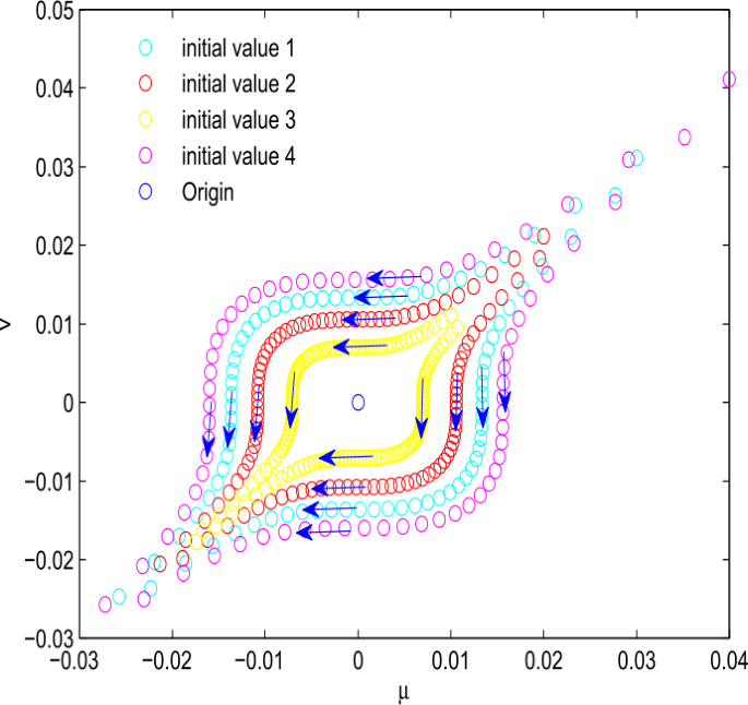

  

  Phase portraits of model (2) near fixed point $\tilde{E}_{0}$

• (2) From Figs. 7 and 8 we can find that the sequence $\{ {{T^{n}}(P)} \} _{0}^{ + \infty }$ enters the third quadrant from the first quadrant along the straight line $\mu =\nu$. In the process the sequence $\{ {{T^{n}}(P)} \} _{0}^{ + \infty }$ is constantly “oscillating” along the straight line $\mu =\nu$, which also confirms Theorem 8.

• (3) Figs. 4, 5, 11, and 12 are very “similar” to subfigures 1, 3, 4−, and F+ of Fig. 8 in [8], respectively, which means that model (2) can have a fold-flip bifurcation near the degenerate fixed point $\tilde{E}_{0}$.

  Figure 5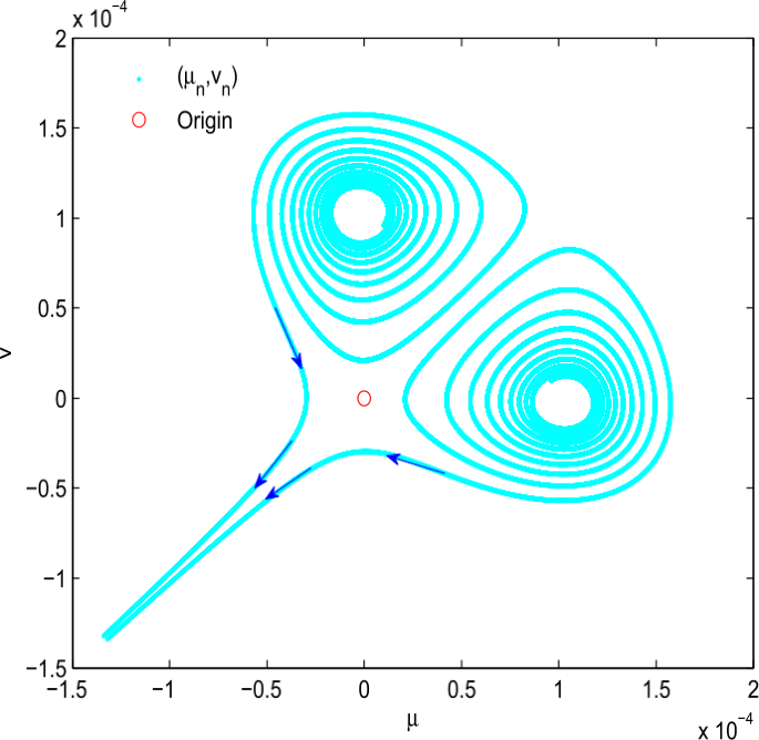

  

  Trajectory of model (1) with the initial value $P_{2}$

Case 1: Suppose the parameters $b=2.0001$ and $d=1$ and the initial value $P_{1}:=(\mu _{0},\nu _{0})=(0.00001,0.0000111)$. Model (2) has fixed points $(0,0)$ and $(2.499875\times 10^{-5}, 2.499875\times 10^{-5})$, and the trajectory of model (2) with initial value $P_{1}$ near the fixed point $(0,0)$ is shown in Fig. 6.

Figure 6

Trajectory of model (2) with the initial value $P_{1}$

Figure 7

Trajectory of model (2) with initial value 4 when $(d,b)=(1,2)$

Case 2: Suppose the parameters $b=2.000434$ and $d=1.00001$ and the initial value $P_{2}:=(\mu _{0},\nu _{0})=(0.00001,0.00096)$. Model (2) has fixed points $(0,0)$ and $(1.109748\times 10^{-5},1.109748\times 10^{-5})$, and the trajectory of model (2) with initial value $P_{2}$ near the fixed point $(0,0)$ is shown in Fig. 5.

Case 3: Suppose the parameter $b=2$ and $d=1$ and the initial value $P_{3}:=(\mu _{0},\nu _{0})=(0.001,0.00111)$. Model (2) has only the fixed point $(0,0)$, and the trajectory of model (2) with initial value $P_{3}$ near the fixed point $(0,0)$ is shown in Fig. 9.

Case 4: Suppose the parameter $d=0.432$ and initial value $(\mu _{0},\nu _{0})=(0.153,0.033)$. The flip bifurcation diagram of model (2) is shown in Fig. 10.

Case 5: Suppose the parameters $b_{1}=2.000105$, $b_{2}=2.00012$, $b_{3}=2.00013$, and $b_{4}=2.00014$. The trajectory of model (2) with initial value $P_{4}:=(\mu _{0},\nu _{0})=(0.00001,0000111)$ is shown in Fig. 11.

Case 6: Suppose the parameters $b_{5}=1.899$, $b_{6}=1.889$, and $b_{7}=1.879$. The trajectory of model (2) with initial value $P_{5}:=(\mu _{0},\nu _{0})=(0.0001,0.000096)$ is shown in Fig. 12.

7 Conclusion

In this paper, we systematically studied bifurcation properties of model (2) near nonhyperbolic fixed points. We obtained the stability and qualitative structures of the degenerate fixed point $\tilde{E}_{0}$. We used the homogeneous polar blowup to study the local behavior of the vector field near the degenerate equilibrium, which avoids complex calculation. By comparing Figs. 5 with Fig. 8 and Fig. 11 with Fig. 12 we can see that the dynamic properties of model (2) vary greatly near $(d, b)=(1,2)$ when the initial value is sufficiently small.

Figure 8

Trajectory of model (2) with initial values 2 and 4 when $(d,b)=(1,2)$

Figure 9

Trajectory of model (2) with the initial value $P_{3}$

Figure 10

Flip bifurcation diagrams of model (2)

Figure 11

Trajectory of model (2) with different parameters b and initial value $P_{4}$

Figure 12

Trajectory of model (2) with different parameters b and initial value $P_{5}$

References

May, R.M.: Simple mathematical models with very complicated dynamics. Nature 261, 459–467 (1976)
Allen, J.S.: Some discrete-time SI, SIR, and SIS epidemic models. Math. Biosci. 124, 83–105 (1994)
Kuznetsov, Y.A.: Elements of Applied Bifurcation Theory, 3rd edn. Springer, New York (2004)
Wiggins, S.: Introduction to Applied Nonlinear Dynamical Systems and Chaos. Springer, New York (1990)
Elaydi, S.: An Introduction to Difference Equations, 3rd edn. Springer, New York (2005)
Guckenheimer, J., Holmes, P.: Nonlinear Oscillations, Dynamical Systems, and Bifurcations of Vector Fields. Springer, New York (1997)
Elaydi, S., Luís, R.: Open problems in some competition models. J. Differ. Equ. Appl. 17, 1873–1877 (2011)
Kuznetsov, Y.A., Meijer, H.G.E., van Veen, L.: The fold-flip bifurcation. Int. J. Bifurc. Chaos 14, 2253–2282 (2004)
Gheiner, J.: Codimension-two reflection and non-hyperbolic invariant lines. Nonlinearity 7, 109–184 (1994)
Meng, L.L., Li, X.F., Zhang, G.: Simple diffusion can support the pitchfork, the flip bifurcations, and the chaos. Commun. Nonlinear Sci. Numer. Simul. 53, 202–212 (2017)
Zeng, L., Zhao, Y., Huang, Y.: Period-doubling bifurcation of a discrete metapopulation model with a delay in the dispersion terms. Appl. Math. Lett. 21, 47–55 (2008)
Gyllenberg, M., Sderbacka, G., Ericsson, S.: Does migration stabilize local population dynamics? Analysis of a discrete metapopulation model. Math. Biosci. 118, 25–49 (1993)
Yakubu, A.A., Castillo-Chavez, C.: Interplay between local dynamics and dispersal in discrete-time metapopulation models. J. Theor. Biol. 218, 273–288 (2002)
Zeng, L., Zhao, Y., Huang, Y.: Hopf bifurcation in a discrete metapopulation model with delay and dispersion. Acta Math. Appl. Sin. 29, 747–754 (2006)
Yuan, L.G., Yang, Q.G.: Bifurcation, invariant curve and hybrid control in a discrete-time predator–prey system. Appl. Math. Model. 39, 2345–2362 (2015)
Chow, S.N., Li, C.Z., Wang, D.: Normal Forms and Bifurcation of Planar Vector Fields. Cambridge University Press, New York (1994)
Zhang, Z.F., Ding, T.R., Huang, W.Z., et al.: Qualitative Theory of Differential Equations. Am. Math. Soc., Providence (1991)
Dumortier, F., Llibre, J., Artés, J.C.: Qualitative Theory of Planar Differential Systems. Springer, Berlin (2006)
Álvarez, M.J., Ferragut, A., Jarque, X.: A survey on the blow up technique. Int. J. Bifurc. Chaos 21, 3103–3118 (2011)
Carr, J.: Applications of Centre Manifold Theory. Springer, New York (1982)
Dumortier, F., Rodrigues, P., Roussarie, R.: Germs of Diffeomorphisms in the Plane. Springer, New York (1981)
Acknowledgements
Not applicable.
Availability of data and materials
Funding
The work is supported by National Natural Science Foundation of China under Grant 11961021 and the Special Funds for the Cultivation of Guangdong College Students’ Scientific and Technological Innovation (No. pdjh2020b0361). The work is also sponsored by Fundation of Graduate Innovation Center in NUAA under Grant Kfjj20190802 and the Innovation and Developing School Project of Guangdong Province under Grant 2019KZDXM032.
Author information
Authors and Affiliations
Contributions
Each of the authors, MSL, XLZ, and JMX, contributed to each part of this study equally and read and approved the final version of the manuscript.
Corresponding author
Ethics declarations
Competing interests
The authors declare that they have no competing interests.
Rights and permissions
Open Access This article is licensed under a Creative Commons Attribution 4.0 International License, which permits use, sharing, adaptation, distribution and reproduction in any medium or format, as long as you give appropriate credit to the original author(s) and the source, provide a link to the Creative Commons licence, and indicate if changes were made. The images or other third party material in this article are included in the article’s Creative Commons licence, unless indicated otherwise in a credit line to the material. If material is not included in the article’s Creative Commons licence and your intended use is not permitted by statutory regulation or exceeds the permitted use, you will need to obtain permission directly from the copyright holder. To view a copy of this licence, visit http://creativecommons.org/licenses/by/4.0/.
About this article
Cite this article
Li, MS., Zhou, XL. & Xu, JM. Dynamic properties of a discrete population model with diffusion. Adv Differ Equ 2020, 580 (2020). https://doi.org/10.1186/s13662-020-03033-w
Received:
Accepted:
Published:
DOI: https://doi.org/10.1186/s13662-020-03033-w