Local fractional system for economic order quantity using entropy solution

Abstract

The economic order quantity (EOQ) model describes the quantity that minimizes the aggregate sum of all cost functions. We propose an assembly for EOQ, nonlinear local fractional differential models with costs functions with respect to time in a cyclic period. For this system, using fractional entropy, we study the related optimization problem and improve a relaxed method for calculating a bounded interval containing the optimal cycle length. Also, for a special class of transportation functions, we study these consequences and introduce processes to compute the optimal size and the matching optimal order stage.

1 Introduction

Recently, the general economy has been defined by an almost linear system. This system must achieve stability. Therefore, it would be difficult to consider its future consequences. In view of the riskiness and complexity typical for this setting, there arises the need to seek out new systems to deal with it. One of the most dynamic features in managing any economic units is the EOQ. In this case, the suggested nonlinear cost function needs to be able to cover all possible properties of the system. These systems are given analytically by suggesting bounded intervals containing an optimal cycle length (reorder interval) to arrive at concave functions [1,2,3,4,5,6], which leads to minimizing the value of EOQ. Other methods of cycle optimal lengths evaluate the upper bound by an algorithm or by utilizing some concepts of convex optimization problems. In our investigation, we introduce some conditions ensuring the boundedness of EOQ by a fractional entropy (Tsallis entropy). Also, we show that this technique minimizes the EOQ by looking for minimal solution.

The notion of local fractional calculus (LFC) was first planned by Kolwankar and Gangal utilizing the Riemann–Liouville fractional derivative. It was realistic to deal with nondifferentiable issues in both science and engineering. Several other ideas of LFC were offered, such as using local fractional derivatives and the fractal geometry (see [7,8,9,10,11]). Moreover, new methods for solving fractal differential equations (numerical and analytic) and real-life applications are provided in [8, 9, 12,13,14].

In this paper, we introduce a nonlinear mathematical system for EOQ. Our tool is a contracting fixed point theorem [15]. Basically, equilibrium theory in economics can be introduced by fixed point theorems. They have been utilized to establish the existence of the set of prices, which are consecutively associated with demand in all markets of an economy (the existence of such prices has been an open question in economics). If this can be done, then the suggested operator has a fixed point according to the theorem. Moreover, the fixed point theorem can be employed to prove the minimum set of fixed points. In our discussion, the minimization of EOQ is described by considering a geometric frame for the total cost function during a time period. We introduce conditions for the existence of solutions for the suggested system, and to obtain an analytic solution, we show that the outcomes of the system are bound by Tsallis fractal entropy.

The advantage of using fractal calculus instead of fractional calculus is that the fractal calculus is known in a fractal space, which has more historical information about an item that is described (variable). Also, since fractal is a self-similar design, it can be easily used in maximization and minimization problems. Fractals also have fractional dimension, and fractals as mathematical arguments cannot be measured by traditional methods, since they are nowhere differentiable. The minimization of EOQ is described by considering a geometric frame for the total cost function during a time period. We introduce conditions for the existence of solutions for the suggested system. We show that the outcomes of the system are bounded by Tsallis entropy.

2 Processing

2.1 LFC

Fractional differential operators without singular kernel were newly studied in [7, 8]. The local fractional derivative of a (fractal) $\phi (\chi )$ of order $0<\alpha \leq 1$ is given by

$$ D^{\alpha } \phi (\chi )= \frac{d^{\alpha } \phi (\chi )}{ \chi ^{\alpha }} \bigg\vert _{\chi =\chi _{0}}= \lim _{\chi \rightarrow \chi _{0}} \frac{d^{\alpha }[\phi (\chi )- \phi (\chi _{0})]}{[d(\chi -\chi _{0})]^{\alpha }}, $$

where the formal $d^{\alpha }[\phi (\chi )-\phi (\chi _{0})]/ [d( \chi -\chi _{0})]^{\alpha }$ is the Riemann–Liouville fractional derivative, which defined by

$$ \frac{d^{\alpha }\phi (\chi )}{d\chi ^{\alpha }}={\frac{1}{\varGamma (1- \alpha )}} {\frac{d}{d\chi }} \int _{0}^{\chi }{\frac{\phi (t)}{(\chi -t)^{ \alpha }}} \,dt; $$

the corresponding integral operator is defined by

$$ \bigl(I^{\alpha }\phi \bigr) (\chi )=\frac{1 }{\varGamma (\alpha )} \int _{0}^{\chi }( \chi -t)^{\alpha -1}\phi (t) \,dt. $$

This operator is well-defined, and it is indicated to the classical fractional calculus. A function ϕ is said to be local fractional continuous at $\chi _{0}$ if for all $\varepsilon >0$, there is κ such that

$$ \bigl\vert \phi (\chi )- \phi (\chi _{0}) \bigr\vert < \varepsilon ^{\alpha } $$

if $\vert \chi -\chi _{0}\vert < \kappa$. We denote the space of all local fractional continuous functions by ${C}_{\alpha }$. For $\phi \in {C}_{\alpha }$, the local fractional integral (LFI) is defined by

$$ I_{[a,b]}^{\alpha } \phi (\varsigma ) = \frac{1}{\varGamma (1+\alpha )} \int ^{b}_{a}\phi (\varsigma ) (d\varsigma )^{\alpha }, $$

where (see [9])

$$ (d\varsigma )^{\alpha }= d^{\alpha }\varsigma = \frac{ \varsigma ^{1-\alpha }}{\varGamma (2-\alpha )} \,d \varsigma ^{\alpha }. $$

Moreover, LFI satisfies the inclusion

$$ I_{[a,b]}^{\alpha }\phi (\varsigma ) \in \biggl[\underline{ \phi } \frac{(b-a)^{ \alpha }}{\varGamma (\alpha +1)}, \bar{\phi } \frac{(b-a)^{\alpha }}{ \varGamma (\alpha +1)}\biggr], $$

where $\underline{ \phi }$ and ϕ̄ are the minimum and maximum values of ϕ, respectively. A necessary and sufficient condition for the existence of the local fractional integral is that a fractal set of local fractional continuity of ϕ has a generalized Lebesgue measure zero. Finally, assume that $\phi (\varsigma ) \in C_{\alpha }[a, b]$. Then there exists a point η in $(a, b)$ such that

$$ I_{[a,b]}^{\alpha } \phi (\varsigma ) = \phi (\eta ) \frac{(b-a)^{ \alpha }}{\varGamma (\alpha +1)}. $$

This implies that

$$ I_{[a,b]}^{\alpha } 1=\frac{(b-a)^{\alpha }}{\varGamma (\alpha +1)}. $$

2.2 EOQ

The model of EOQ was given by Harris [16] as follows:

$$ Q= \sqrt{2AB/ C}, $$

(1)

where A is the annual demand quantity, B is the fixed cost per item, and C is the annual holding cost per item. In [17] the authors suggested that (1) changes over time as follows:

$$ \begin{aligned} \frac{d}{d \tau }Q(\tau ) &= Q(\tau ) G( \tau , A,B,C). \end{aligned} $$

(2)

Equation (2) is a general case of the suggested model (differential EOQ) given in [18].

In this section, we study the local fractional system (LFS)

$$ \begin{aligned} D^{\alpha }Q(\tau )= F \bigl(\tau , \tau Q(\tau ), \tau Q(a \tau ), \tau Q(b \tau ),\tau Q(c \tau ) \bigr) , \end{aligned} $$

(3)

where a, b, and c are nonnegative constants referring to the average changes in A, B, and C, respectively.

Definition 1

Let $(\mathbb{B}, \Vert \cdot \Vert )$ be a Banach space over $\mathbb{R}$. A function $F: \mathbb{R}^{5}_{+} \longrightarrow \mathbb{B}$ is homogeneous of order $0 \leq \epsilon <1$ with respect to $\tau \in \mathbb{R}_{+}$ if

$$ F \bigl(\tau , \tau Q(\tau ), \tau Q(a \tau ), \tau Q(b \tau ),\tau Q(c \tau ) \bigr):= \tau ^{\epsilon }F \bigl( Q_{0}(\tau ), Q_{1}( \tau ), Q _{2}( \tau ), Q_{3}( \tau ), Q_{4}( \tau ) \bigr). $$

In economic philosophy, we suppose that a company’s manufacture function is homogeneous of degree 1 (if all efforts are grown by τ, then production is multiplied by τ). A production function with this possession is said to assign fixed scale.

Another example: assume that a user’s demand for goods, as a function of values and her income, stands up from her selection among all the bundles she can give, the one that is best giving to her favorites. Then we can impose that this demand function is homogeneous of degree zero: if all costs and the user’s profits are multiplied by any number $\tau > 0$, then her demands for goods remain the same.

Definition 2

Let the function $F, Q \in C_{\alpha }$ be fractional continuous with respect to $\tau \in \mathbb{R}_{+}$. Then F is called a generalized Lipschitz function (GLF) with respect to $Q_{i}$, $i=0,\ldots,4$, if there is a positive constant $\wp > 0$ such that

$$ \begin{aligned} & \bigl\Vert F \bigl( Q_{0}(\tau ), Q_{1}(\tau ), Q_{2}( \tau ), Q_{3}( \tau ), Q _{4}( \tau ) \bigr)- F \bigl( \mathfrak{Q}_{0}(\tau ), \mathfrak{Q}_{1}( \tau ), \mathfrak{Q}_{2}( \tau ), \mathfrak{Q}_{3}( \tau ), \mathfrak{Q}_{4} (\tau ) \bigr) \bigr\Vert \\ & \quad \leq \wp ^{\alpha } \bigl( \Vert Q_{0}- \mathfrak{Q}_{0} \Vert + \Vert Q_{1}- \mathfrak{Q}_{1} \Vert + \Vert Q_{2}- \mathfrak{Q}_{2} \Vert + \Vert Q_{3}- \mathfrak{Q}_{3} \Vert + \Vert Q_{4}- \mathfrak{Q}_{4} \Vert \bigr) \\ &\quad = \wp ^{\alpha }\sum^{4}_{i=0} \Vert Q_{i}- \mathfrak{Q}_{i} \Vert \\ &\quad \leq 5 \wp ^{\alpha } \Vert Q- \mathfrak{Q} \Vert := \varrho \Vert Q- \mathfrak{Q} \Vert , \quad \varrho := 5 \wp ^{\alpha }. \end{aligned} $$

Definition 3

Let $\mathbb{B}: = C_{\alpha }$ be a generalized Banach space with norm $\Vert \cdot \Vert _{\alpha }$, and let $\varPhi : \mathbb{B} \longrightarrow \mathbb{B}$. If $\phi \in \mathbb{B}$ satisfies $\Vert \varPhi \phi ^{\alpha }- \phi ^{\alpha }\Vert _{\alpha }=0$, then $\phi ^{\alpha }$ is called a fixed point of Φ. Moreover, if

$$ \bigl\Vert \varPhi \phi ^{\alpha }-\varPhi \psi ^{\alpha } \bigr\Vert _{\alpha }\leq \lambda ^{\alpha } \bigl\Vert \phi ^{\alpha }- \psi ^{\alpha } \bigr\Vert _{\alpha } $$

for $\psi \in \mathbb{B}$,then Φ is called a contraction mapping. It is well known that a contracting mapping Φ on $\mathbb{B}$ has a unique fixed point.

In our study, we consider the system

$$\begin{aligned}& \begin{aligned}[b] &D^{\alpha }Q(\tau )= \tau ^{\epsilon }F \bigl( Q_{0}(\tau ), Q_{1}( \tau ), Q_{2}( \tau ), Q_{3}( \tau ), Q_{4}( \tau ) \bigr) \\ &\quad ( \tau \geq 0, 0\leq \epsilon < 1 ), \end{aligned} \end{aligned}$$

(4)

where F is a GLF. Define the operator $\varPhi : \mathbb{B} \rightarrow \mathbb{B}$ by

$$\begin{aligned}& \varPhi Q(\tau )= q_{0}+ \frac{1}{\varGamma (1+\alpha )} \int ^{1}_{0} \tau ^{\epsilon }F \bigl( Q_{0}(\tau ), Q_{1}(\tau ), Q_{2}( \tau ), Q _{3}( \tau ), Q_{4}( \tau ) \bigr) (d\tau )^{\alpha } \\& \quad \bigl(\tau \in J:=[0,1], 0 < \alpha < 1, Q(0)=q_{0} \bigr). \end{aligned}$$

(5)

2.3 Local fractional entropy (LFE)

Tsallis presented an entropic formalization characterized by an index γ that implies a nonextensive statistics. The Tsallis entropy ($\mathbb{T}_{\gamma }$) is the basis of the so known nonextensive statistical mechanics, which modifies the Boltzmann–Gibbs theory. The Tsallis statistics has been used in various fields such as applied mathematics, applicable mathematics, physics, biology, chemistry, computer science, information theory, engineering, medicine, economics, business, geophysics, and so on. The general continuous form of this entropy is given by

$$ \mathbb{T}_{\gamma }(\varphi )= \frac{ \int _{x} ( \varphi (x))^{ \gamma }\,dx-1}{1-\gamma }, \quad \gamma \neq 1. $$

Let $x=\tau ^{\alpha }$. Then we have the LFE

$$ \mathbb{T}^{\alpha }_{\gamma }(\varphi )= \frac{ \int _{\tau }( \varphi (\tau ^{\alpha }))^{\gamma }\,d \tau ^{\alpha }-1}{1-\gamma }. $$

We prove that a unique solution of Eq. (4) is bounded by the Tsallis entropy under some assumptions. This solution minimizes the EOQ.

2.4 Preliminary

We need the following result.

Lemma 1

(Leray–Schauder theorem)

Let Π be a continuous compact mapping of a Banach space ${ \mathbb{B}}$ into itself such that the set

$$ \{\xi \in \mathbb{B}: \xi =\lambda \varPi \xi {\textit{ for some }}0\leq \lambda \leq 1\} $$

is bounded. Then Π has a fixed point.

3 Results

In this section, we introduce two cases of the function F in (4).

Let the functions F and Q be continuous with respect to $\tau \in J=[0,1]$, and let F be Lipschitz with respect to $Q_{i}$, $i=0,\ldots,4$, such that $F(0)=f_{0}$, $f_{0} \in \mathbb{R} _{+}$. Define the operator Φ as in (5).

We have the following results.

Theorem 1

Consider Eq. (4). If for $\varrho >0$ and $0< \alpha <1$,

$$ \frac{\varrho }{\varGamma (2-\alpha )\varGamma (1+\alpha )} < 1, $$

then it admits a unique solution that minimizes problem (4).

Proof

Obviously,

$$ \begin{aligned} \bigl\vert (\varPhi ) (Q) (\tau ) \bigr\vert &= \biggl\vert q_{0}+ \frac{1}{\varGamma (1+\alpha )} \int ^{1}_{0} \tau ^{\epsilon }F \bigl( Q_{0}(\tau ), Q_{1}(\tau ), Q_{2}( \tau ), Q_{3}( \tau ), Q_{4}( \tau ) \bigr) (d\tau )^{\alpha } \biggr\vert \\ &\leq q_{0}+ \frac{1}{\varGamma (1+\alpha )} \int ^{1}_{0} \tau ^{\epsilon } \bigl( \bigl\vert F \bigl( Q_{0}(\tau ), Q_{1}(\tau ), Q_{2}( \tau ), Q_{3}( \tau ), Q_{4}( \tau ) \bigr) \\ &\quad{} -F(0) \bigr\vert + \vert f_{0} \vert \bigr) (d\tau )^{\alpha } \\ &\leq q_{0}+\frac{1}{\varGamma (2-\alpha )\varGamma (1+\alpha )}\bigl(\varrho \Vert Q \Vert +f_{0}\bigr) \int ^{1}_{0} \tau ^{\epsilon +1-\alpha }\,d \tau ^{\alpha }. \end{aligned} $$

Since $\max_{J}\{\tau ^{\epsilon +1-\alpha }\}=1$, we have

$$ \Vert Q \Vert \leq \frac{q_{0}+ \frac{f_{0}}{\varGamma (2-\alpha )\varGamma (1+ \alpha )}}{1- \frac{\varrho }{\varGamma (2-\alpha )\varGamma (1+\alpha )}}. $$

The operator Φ is continuous, bounded, and compact in a subset of the Banach space $\mathbb{B}$. Hence, in view of Lemma 1, system (4) has a solution. A calculation implies that

$$ \begin{aligned} \bigl\vert (\varPhi ) (Q) (\tau )-(\varPhi ) (\mathfrak{Q}) (\tau ) \bigr\vert &\leq \frac{1}{\varGamma (1+\alpha )} \int ^{1}_{0} \tau ^{\epsilon } \bigl\vert F \bigl( \mathbf{Q}(\tau )\bigr)- F\bigl( \mathfrak{Q} ( \tau )\bigr) \bigr\vert (d \tau )^{\alpha } \\ &\leq \frac{\varrho }{\varGamma (2-\alpha )\varGamma (1+\alpha )} \Vert Q- \mathfrak{Q} \Vert . \end{aligned} $$

If $\frac{\varrho }{\varGamma (2-\alpha )\varGamma (1+\alpha )} <1$, then Φ is a contraction mapping, and we conclude that (4) has a unique solution. It is clear that the fixed point corresponds to equilibrium of EOQ. □

Theorem 2

Let F be a homogeneous function achieving (4) and suppose that for $0< \gamma <1$ and $0< \alpha <1$,

$$ \Vert F \Vert \leq \frac{\varGamma (2-\alpha )\varGamma (1+\alpha )}{1-\gamma }, \quad \gamma \neq 1. $$

If $q_{0} > 1/ \gamma$, then every solution of (4) taking formula (5) is bounded by local fractional entropy for all $\tau \in J$.

Proof

Let Q be a solution of the form

$$ Q(\tau )= q_{0}+ \frac{1}{\varGamma (1+\alpha )} \int ^{1}_{0} \tau ^{\epsilon }F \bigl( Q_{0}(\tau ), Q_{1}(\tau ), Q_{2}( \tau ), Q _{3}( \tau ), Q_{4}( \tau ) \bigr) (d\tau )^{\alpha }. $$

The function F satisfies

$$ F \bigl(\tau , \tau Q(\tau ), \tau Q(a \tau ), \tau Q(b \tau ),\tau Q(c \tau ) \bigr)= \tau ^{\epsilon }F \bigl( Q_{0}(\tau ), Q_{1}(\tau ), Q _{2}( \tau ), Q_{3}( \tau ), Q_{4}( \tau ) \bigr), $$

which implies

$$ F \bigl( Q_{0}(\tau ), Q_{1}(\tau ), Q_{2}( \tau ), Q_{3}( \tau ), Q _{4}( \tau ) \bigr)= \frac{F (\tau , \tau Q(\tau ), \tau Q(a \tau ), \tau Q(b \tau ),\tau Q(c \tau ) )}{ \tau ^{\epsilon }}. $$

Suppose that $\tau = \frac{1}{ Q_{0}(\tau )}$. Then we have

$$\begin{aligned}& F \bigl( Q_{0}(\tau ), Q_{1}(\tau ), Q_{2}( \tau ), Q_{3}( \tau ), Q _{4}( \tau ) \bigr) \\& \quad = Q_{0}(\tau ) ^{\epsilon } F \biggl( \frac{1}{Q _{0}(\tau )}, \frac{Q_{1}(\tau )}{Q_{0}(\tau )}, \frac{Q_{2}(\tau )}{Q _{0}(\tau )}, \frac{Q_{3}(\tau )}{Q_{0}(\tau )}, \frac{Q_{4}(\tau )}{Q _{0}(\tau )} \biggr). \end{aligned}$$

A computation implies that

$$\begin{aligned} Q(\tau ) &= q_{0}+ \frac{1}{\varGamma (1+\alpha )} \int ^{1}_{0}Q _{0}(\tau ) ^{\epsilon } F \biggl( \frac{1}{Q_{0}(\tau )}, \frac{Q _{1}(\tau )}{Q_{0}(\tau )}, \frac{Q_{2}(\tau )}{Q_{0}(\tau )}, \frac{Q _{3}(\tau )}{Q_{0}(\tau )}, \frac{Q_{4}(\tau )}{Q_{0}(\tau )} \biggr) (d\tau )^{\alpha } \\ &\leq q_{0}+ \frac{ \Vert F \Vert }{\varGamma (2-\alpha )\varGamma (1+\alpha )} \int ^{1}_{0} Q_{0}(\tau ) ^{\epsilon }\tau ^{1-\alpha } \,d\tau ^{\alpha } \\ &= q_{0}+ \frac{ \Vert F \Vert }{\varGamma (2-\alpha )\varGamma (1+\alpha )} \int ^{1}_{0} \frac{Q_{0}(\tau ) ^{\epsilon -1}}{ \tau ^{\alpha }} \,d \tau ^{\alpha } \\ &\leq q_{0}+ \frac{1}{1-\gamma } \int ^{1}_{0} \mathbf{Q}_{0}\bigl( \tau ^{\alpha }\bigr) ^{\gamma } \,d\tau ^{\alpha }, \quad \gamma := \epsilon -1>0, \mathbf{Q}_{0}=\frac{Q_{0}(\tau ) }{ \tau ^{\alpha /\gamma }} \\ &= \frac{q_{0}- q_{0} \gamma }{1-\gamma }+\frac{\int ^{1}_{0} \mathbf{Q}_{0}(\tau ^{\alpha }) ^{\gamma } \,d\tau ^{\alpha }}{1-\gamma }. \end{aligned}$$

Since $q_{0}> 1/\gamma$, we obtain the following inequality:

$$ Q(\tau ) \leq \frac{q_{0}}{1-\gamma } + \frac{\int ^{1}_{0} \mathbf{Q}_{0}(\tau ^{\alpha }) ^{\gamma } \,d\tau ^{\alpha }-1}{1-\gamma }, \quad \tau \in J. $$

Hence every solution of (4) is bounded by LFE. □

4 Examples

In this section, we consider some applications.

Example 1

Assume that a company’ s production in two seasons during a year achieves the EOQ system, where $\mathbf{Q}_{0}(\tau ^{\alpha }) =1$, $\tau _{1}, \tau _{2} \in J=[0,1]$, and $\gamma =0.5$:

$$ \begin{aligned} & Q(\tau _{1})= \frac{1}{1-\gamma }\bigl[A(1)B(1)-C(1) Q(2)\bigr], \\ & Q(\tau _{2})=\frac{1}{1-\gamma }\bigl[A(2)B(2)-C(2) Q(1)\bigr]. \end{aligned} $$

(6)

Define the company’ s reaction function $\rho :\mathbb{R}^{2}_{+} \rightarrow \mathbb{R}^{2}_{+}$ by

$$ \rho \bigl( Q(\tau _{1}), Q(\tau _{2})\bigr) := \frac{1}{1-\gamma } \bigl(A(1)B(1)-C(1) Q(\tau _{2}), A(2)B(2)-C(2) Q( \tau _{1}) \bigr). $$

If $\max \{C(1),C(2)\}<1$, then a computation with respect to city block metric yields

$$ \begin{aligned} \bigl\vert \rho ( \mathbf{Q}) - \rho \bigl( \mathbf{Q}^{\prime }\bigr) \bigr\vert &=\frac{1}{1- \gamma } \bigl\vert A(1)B(1)-C(1) Q(\tau _{2})- \bigl(A(1)B(1)-C(1) Q^{\prime }(\tau _{2}) \bigr) \bigr\vert \\ &\quad{} + \frac{1}{1-\gamma } \bigl\vert A(2)B(2)-C(2) Q(\tau _{1})- \bigl( A(2)B(2)-C(2) Q^{\prime }(\tau _{1}) \bigr) \bigr\vert \\ &=\frac{1}{1-\gamma }\bigl[ C(1) \bigl\vert Q^{\prime }(\tau _{2})-Q(\tau _{2}) \bigr\vert + C(2) \bigl\vert Q ^{\prime }(\tau _{1})-Q(\tau _{1}) \bigr\vert \bigr] \\ &\leq \frac{1}{1-\gamma }\max \bigl\{ C(1),C(2)\bigr\} \bigl( \bigl\vert Q^{\prime }(\tau _{2})-Q(\tau _{2}) \bigr\vert + \bigl\vert Q^{\prime }(\tau _{1})-Q(\tau _{1}) \bigr\vert \bigr) \\ &=\frac{1}{1-\gamma } \max \bigl\{ C(1),C(2)\bigr\} \bigl\vert \mathbf{Q}-\mathbf{Q}^{ \prime } \bigr\vert . \end{aligned} $$

Thus the existence and uniqueness outcome for the equilibrium, where ρ has a unique fixed point $\mathbf{Q}^{*}$ if $C(i)<1$, $i=1,2$. We have the following facts:

• The condition $C(i)<1-\gamma$, $i=1,2$, is sufficient for equilibrium but not necessary.

• In view of the condition $C(i)<1-\gamma$, $i=1,2$, system (6) can be considered as a fuzzy system with different values of $0<\gamma < 1$ (see Fig. 1).

  Figure 1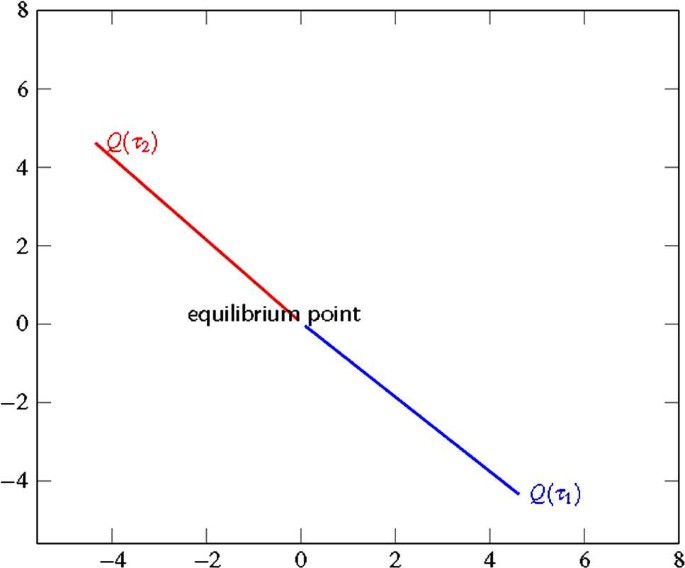

  

  Example 1; The behavior of local fractional entropy for functions $Q(\tau _{1})$ in the horizontal axis and $Q(\tau _{2})$ in the vertical axis. Here, we suppose $\alpha = 0.95$, $C(i) = 0.499< 0.5$, $i =1,2$, and $A(i) = 0.1$, $B(i) = 0.3$. This shows that the entropy solution is a unique solution for the system (6). Moreover, the equilibrium point is at the origin $(0,0)$. Note that when $\alpha \to 0$, the system will loss its equilibrium

Example 2

Assume that a recent state of market is $Q(0)=(Q_{1}(0),Q_{2}(0))$. A company j is imposing $\mathbf{Q}_{0}(\tau ^{\alpha }) =1$ units. At time $\tau =1$, each company selects its outcome level $Q_{j}(1)$ by replaying to the quantity. Consequently, we have the system (see Fig. 2)

$$ \begin{aligned} &Q_{1} (1)=\frac{1}{1-\gamma } \bigl[A(1)B(1) -C(1)Q_{2} (\tau )\bigr], \quad \tau \in J=[0,1], \\ & Q_{2} (1)=\frac{1}{1-\gamma }\bigl[A(2)B(2) -C(2)Q_{1} ( \tau )\bigr]. \end{aligned} $$

(7)

The sequence $\langle Q(\tau )\rangle$ converges to the equilibrium point $Q^{*}$ whenever $\max \{C(1), C(2)\}<1-\gamma$, $0< \gamma <1$.

Figure 2

Example 2; The local entropy solution for a function $\alpha = 0.99$, $Q(\tau ) = (Q_{1},Q_{2})$ with respect to τ. We suppose $C(1) = 0.499$, $C(2) = 0.2$

Example 3

Consider the following nonlinear system:

$$ \begin{aligned} &Q_{1} (\tau )= \frac{1}{2(1-\gamma )(1+Q_{2} (\tau ))}, \\ & Q_{2} (\tau )=\frac{\exp (- Q_{1} (\tau ))}{2(1-\gamma )}. \end{aligned} $$

(8)

It is clear that the function $\varTheta : \mathbb{R}^{2}_{+} \rightarrow \mathbb{R}^{2}_{+}$ defined as

$$ \varTheta (Q_{1},Q_{2}) = \biggl( \frac{1}{2(1-\gamma )(1+Q_{2} (\tau ))}, \frac{\exp (- Q_{1} (\tau ))}{2(1-\gamma )} \biggr) $$

is a contraction mapping with a contraction constant $1/(2(1-\gamma ))<1$. This implies that $\gamma < 0.5$, so that an equilibrium point exists and is unique (see Fig. 3).

Figure 3

Example 3: the functions $\alpha = 0.88$, $Q(\tau )$ with respect to τ. There is a unique equilibrium point for the system corresponding to a unique solution

Example 4

Consider the following nonlinear equation $Q: J \rightarrow \mathbb{R}_{+}$:

$$ Q(\tau )= \frac{1}{2(1-\gamma )} \biggl( \tau + C \frac{1}{\tau } \biggr), \quad \tau \neq 0. $$

(9)

It is clear that $\lim_{\tau \longrightarrow 0} Q(\tau )=\infty$. To minimize (9), we use an approximation technique. The approximation form of (9) is as follows:

$$ \tau _{m+1} =\frac{1}{2(1-\gamma )} \biggl( \tau _{m}+ C \frac{1}{\tau _{m}} \biggr), \quad \gamma < 0.5. $$

(10)

It is clear that this sequence converges to $\sqrt{C}$. Therefore, since $Q(\tau )$ is continuous, $\sqrt{C}$ is a fixed point of Q. Also, in view of Theorem 1, for $0< \sqrt{C}<1$, Eq. (9) has a unique fixed point corresponding to the solution of it. The reaction of (10) showed that it has a limit and this limit converges to the fixed point of (9). Therefore there is no need to show that the function Q is a contraction mapping.

5 Discussion

In general, economics can be performed by a set of fixed points; thus fixed point theorems can provide equilibria of economics together with the local fractional entropy (as an upper bound for the solution). The frame of this work was to consider a new formula of the EOQ model. We introduced a technique of minimizing it by using the concept of fixed point theory. We developed this method to be suitable to the model (see Theorem 1). Applications are given, including linear and nonlinear systems. These systems are based on changing the solution during a fixed time interval. The equilibrium points of each system were established, where it represented by the stationary state at which the markets clear. Also, this stationary state acted when the company wanted to change its strategy.

References

Grubbstrom, R.W.: Modelling production opportunities an historical overview. Int. J. Prod. Econ. 41, 1–14 (1995)
Caplin, A., Leahy, J.: Economic theory and the world of practice: a celebration of the \((S, s)\) model. J. Econ. Perspect. 24(1), 183–201 (2010)
Malakooti, B.: Operations and Production Systems with Multiple Objectives. Wiley, New York (2013). ISBN 978-1-118-58537-5
Holmbom, M., Segerstedt, A.: Economic order quantities in production: from Harris to economic lot scheduling problems. Int. J. Prod. Econ. 155, 82–90 (2014)
Lagodimos, A.G., et al.: The discrete-time EOQ model: solution and implications. Eur. J. Oper. Res. 266(1), 112–121 (2018)
Ibrahim, R.W., et al.: Fractional differential texture descriptors based on the Machado entropy for image splicing detection. Entropy 17(7), 4775–4785 (2015)
Caputo, M., Fabrizio, M.: A new definition of fractional derivative without singular kernel. Prog. Fract. Differ. Appl. 1(2), 73–85 (2015)
Yang, X., Baleanu, D., Srivastava, H.M.: Local Fractional Integral Transforms and Their Applications. Elsevier, Amsterdam (2016)
Cattani, C., Srivastava, H.M., Yang, X.-J.: Fractional Dynamics. de Gruyter, Berlin (2015)
Su, W., Yang, X., Jafari, H., Baleanu, D.: Fractional complex transform method for wave equations on Cantor sets within local fractional differential operator. Adv. Differ. Equ. 2013, 97 (2013)
Kalamani, P., Baleanu, D., Arjunan, M.M.: Local existence for an impulsive fractional neutral integro-differential system with Riemann–Liouville fractional derivatives in a Banach space. Adv. Differ. Equ. 2018, 416 (2018)
Yang, X.-J., Gao, F., Srivastava, H.M.: A new computational approach for solving nonlinear local fractional PDEs. J. Comput. Appl. Math. 339, 285–296 (2018)
Yang, X.-J., Baleanu, D., Gao, F.: New analytical solutions for Klein–Gordon and Helmholtz equations in fractal dimensional space. Proc. Rom. Acad., Ser. A: Math. Phys. Tech. Sci. Inf. Sci. 18(3), 231–238 (2017)
Yang, X.-J., et al.: Exact travelling wave solutions for local fractional partial differential equations in mathematical physics. In: Mathematical Methods in Engineering, pp. 175–191. Springer, Cham (2019)
Jafari, H., Jassim, H.K., Al Qurashi, M., Baleanu, D.: On the existence and uniqueness of solutions for local fractional differential equations. Entropy 18(11), 420 (2016)
Harris, R.W.: How many parts to make at once. Oper. Res. 38(6), 947 (1990)
Ibrahim, R.W., Hadid, S.B.: The EOQ model: a differential cyclic system for calculating economic order quantity. Int. J. Anal. Appl. 16(3), 437–444 (2018)
Mahata, G., Mahata, P.: Analysis of a fuzzy economic order quantity model for deteriorating items under retailer partial trade credit financing in a supply chain. Math. Comput. Model. 53, 1621–1636 (2011)
Acknowledgements
The authors thank the referee for careful reading and helpful suggestions on the improvement of the manuscript.
Funding
No funding was received.
Author information
Authors and Affiliations
Contributions
All authors contributed equally and read and approved the final version of the manuscript.
Corresponding author
Ethics declarations
Competing interests
The authors declare that there is no conflict of interests regarding the publication of this manuscript. The authors declare that they have no competing interests.
Additional information
Publisher’s Note
Springer Nature remains neutral with regard to jurisdictional claims in published maps and institutional affiliations.
Rights and permissions
Open Access This article is distributed under the terms of the Creative Commons Attribution 4.0 International License (http://creativecommons.org/licenses/by/4.0/), which permits unrestricted use, distribution, and reproduction in any medium, provided you give appropriate credit to the original author(s) and the source, provide a link to the Creative Commons license, and indicate if changes were made.
About this article
Cite this article
Ibrahim, R.W., Jafari, H., Jalab, H.A. et al. Local fractional system for economic order quantity using entropy solution. Adv Differ Equ 2019, 96 (2019). https://doi.org/10.1186/s13662-019-2033-4
Received:
Accepted:
Published:
DOI: https://doi.org/10.1186/s13662-019-2033-4