Some new solutions of the Caudrey–Dodd–Gibbon (CDG) equation using the conformable derivative

Abstract

New exact solutions of the space–time conformable Caudrey–Dodd–Gibbon (CDG) equation have been derived by implementing the conformable derivative. The generalized Riccati equation mapping method is applied to figure out twenty-seven forms of exact solutions, which are soliton, rational, and periodic ones. Also, for some suitable values of parameters, the exact solutions are found, namely dark, bell type, periodic, soliton, singular soliton, and several others, by using the conformable derivative. These types of solutions have not been proclaimed so far. 2D and 3D graphical patterns of some solutions are also given for clarification of physical features. The conformable derivative is one of the excellent choices to solve the nonlinear conformable problems arising in theory of solitons and many other areas. The results are new and very interesting for the large community of researchers working in the field of mathematics and mathematical physics.

1 Introduction

Fractional calculus [1, 2] containing differential equations of fractional order in numerous physical phenomena has put a revolutionary impact since these particular equations reflect generalization of evolution equations of integer order. Derivatives and integrals of real fractional order or complex order can be applied in many fields. These fields are geochemistry, plasma physics, mechanics, control theory, optical fibers, solid state physics, system identification, chemical kinematics, biogenetics, etc. These phenomena involve diffusion, dispersion, dissipation convection, and reaction.

Finding the extraction of exact traveling wave solutions of nonlinear differential equations has become very important for discussing wave phenomena of nonlinear nature. Many analytical, approximate and numerical techniques have been used for finding exact solutions of nonlinear differential equations including homotopy analysis transform method [3], homotopy analysis samadu transform method [4], fractional homotopy analysis transform method [5], the differential transform method [6], F-expansion method [7], first integral method [8], fractional sub-equation method [9], sine-cosine method [10], variational iteration method [11, 12], exponential rational function method [13, 14], exp-function method [15,16,17,18], $( \frac{G'}{G} )$-expansion method [19,20,21], $\exp (- \phi (\xi ))$-expansion method [22], $\tan( \frac{ \varPhi ( \xi )}{2} )$ expansion method [23, 24], modified trial equation method [25, 26], etc. Some recent advancements include fractional nonlinear dynamics [27], new fractional order view of HIV and CD4+ T-cells [28], life cycle involving poor nutrition [29], and control theory [30]. Further, a new analysis regarding Mittag-Leffler type kernel [31], study of computer viruses [32] are the recent advancements in fractional derivatives and their applications.

To seek out exact solutions of some nonlinear evolutions equations (NEEs), a Riccati equation mapping method is introduced by considering the nonlinear ODE: $\varphi ( \xi ) = r + p\varphi ( \xi ) + q \varphi ^{2} ( \xi )$. This approach was formulated from the $( \frac{G'}{G} )$ method by utilizing Cole–Hopf transformation and yielded many solutions as compared to the $( \frac{G'}{G} )$-expansion method. The generalized Riccati equation mapping is simple, straightforward, convenient for homogeneous balancing order and in working out a system of algebraic equations and can produce a variety of exact solutions of differential equations. This work discovers twenty-seven types of different solutions comprising hyperbolic, periodic, and rational solutions.

In [33], Khalil introduced the notion of conformable derivative, suitably compatible with integer order derivative and satisfying some conventional properties such as the chain rule. Atangana discussed some features of this particular derivative in [34]. The author presented proofs of linked theorems and gave new definitions. This operator is also investigated in [35, 36], leading to fruitful discussion. By using sub-equation method in conjunction with conformable operator, Rezazadeh in [37] found solutions of traveling wave form for conformable generalized Kuramoto–Sivashinsky equation. The resulting solutions were presented in hyperbolic and trigonometric forms. In [38], the authors extracted exact solutions of conformable regularized long-wave equations, while some other analytical techniques are given in [39, 40]. A new form of conformable derivative is proposed by Atangana [41] referred to as beta fractional operator, overcoming the limitation of conformable derivative.

In this work, we focus on the relatively modern fractional differentiation known as Atangana–Baleanu fractional differentiation [42]. Abdon Atangana, an African researcher and mathematician, presented his new idea of fractional operators. This particular work attracted many investigators to apply it to a number of problems of practical applications. Atangana et al. gave new properties of the conformable fractional operator or derivative. Abdon Atangana and Dumitru Baleanu studied the Mittag-Lefler function which is a more generalized function. Consequently, they introduced a fractional derivative, based on non-local kernel, describing complex nonlinear applied problems of complex nature. The power and exponential decay law was also considered. This new version derivative is found to be more appealing and advantageous than the already established ones.

The solutions of space–time conformable Caudrey–Dodd–Gibbon (CDG) equation are sought by different methods, e.g., Wazwaz [43] used the tanh method to obtain solitary wave solutions. Zhou et al. [44] applied the exp-function method to derive generalized solitary solution. In 2011 [45], the authors obtained traveling wave solutions by the $( \frac{G'}{G} )$-expansion method. By studying the generalized Riccati equation mapping method [46], the conformable derivative of Atangana’s version finds the hyperbolic, rational, and trigonometric solutions of (CDG) equation, not brought to light before in the literature so far. Next section therefore gives some new solutions of traveling wave form of the space–time conformable Caudrey–Dodd–Gibbon (CDG) equation.

Analysis of the generalized Riccati equation mapping is presented in Sect. 2. We have implemented the same mapping for attaining new exact soliton solutions to the time and space conformable Caudrey–Dodd–Gibbon (CDG) equation in Sect. 3. Physical interpretation and comparison will be presented in Sects. 4 and 5, whereas the last section includes our conclusion.

2 The improved generalized Riccati equation mapping method

The focal steps of this technique [47,48,49] are as follows.

Step 1. We consider the conformable differential equation including independent variables $x_{1}, x_{2},\ldots, x_{m}$, t and some unknown function u:

$$ p \bigl( u, {}_{0}^{A} D_{t}^{\alpha } u, {}_{0}^{A} D_{x_{1}}^{ \alpha } u, {}_{0}^{A} D_{x_{2}}^{\alpha } u, {}_{0}^{A} D_{x_{3}} ^{\alpha } u,\ldots, {}_{0}^{A} D_{t}^{2 \alpha } u, {}_{0}^{A} D _{x_{1}}^{2 \alpha } u, {}_{0}^{A} D_{x_{2}}^{2 \alpha } u,\ldots \bigr) =0, $$

(1)

where ${}_{0}^{A} D_{t}^{\alpha }$ and ${}_{0}^{A} D_{x}^{\alpha }$ are known as Atangana’s conformable differential operators.

Step 2. For the said operator, we use the variable transformation:

$$ \begin{gathered} u ( x_{1}, x_{2},\ldots, x_{m}, t ) = U ( \xi ), \\ \begin{aligned} \xi &= \frac{\chi 1}{\alpha } \biggl( x_{1} + \frac{1}{\varGamma ( \alpha )} \biggr)^{\alpha } + \frac{\chi 2}{\alpha } \biggl( x _{2} + \frac{1}{\varGamma ( \alpha )} \biggr)^{\alpha } + \cdots + \frac{\chi m}{\alpha } \biggl( x_{m} + \frac{1}{\varGamma ( \alpha )} \biggr)^{\alpha } \\ &\quad{} + \frac{\lambda }{\alpha } \biggl( t + \frac{1}{\varGamma ( \alpha )} \biggr)^{\alpha }, \end{aligned} \end{gathered} $$

(2)

where the constants λ and χi are to be determined. The conformable differential equation (1) leads to the nonlinear conformable ODE for $u ( x, t ) = u ( \xi )$:

$$ R =R \bigl( u ( \xi ), u' ( \xi ), u^{\prime \prime } ( \xi ),\ldots \bigr) =0, $$

(3)

where $u' ( \xi ) = \frac{du ( \xi )}{d \xi }$ indicates a derivative in terms of ξ.

Step 3. We consider an assumption that the solution of Eq. (3) can be given by a polynomial in $\phi (\xi )$ as follows:

$$ u ( \xi ) = \sum_{i=-n}^{n} a_{i} \phi (\xi )^{i}, $$

(4)

where $a_{i}$ ($i=0,\pm 1,\pm 2,\ldots,\pm n$) are constants, which are to be determined provided $a_{i} \neq 0$. The function $\phi =\phi ( \xi )$ satisfies the Riccati differential equation [49]

$$ \phi ' ( \xi ) =r+p\phi ( \xi ) +\phi ( \xi )^{2}. $$

(5)

Step 4. Positive integer N is found by using homogeneous balance between the nonlinear term and the highest order derivatives in Eq. (3).

Step 5. Plugging Eq. (4) along with Eq. (5) into Eq. (3), followed by collecting all the same order terms $\phi ^{i}$ together, we get the polynomial equation in $\phi ^{i}$ and $\phi ^{-i}$, where ($i=0,1,2,\ldots$). Equalizing coefficients of the resulting polynomial to zero, we get an over-determined system of algebraic equations for $a_{i}$, where $i=0,\pm 1,\pm 2,\ldots,\pm n$.

Step 6. By using Maple, we work out the system described in Step 5 for obtaining $a_{i}$, where $i =0,\pm 1,\pm 2,\ldots,\pm n$. We plug the obtained values in Eq. (4) along with solutions of Eq. (5) using the transformation in Eq. (2) to obtain several exact solutions of Eq. (1). For general solutions of Eq. (1), the generalized Riccati equation mapping technique gives twenty-seven solutions of the Riccati equation in Eq. (5) presenting four different families [49] as follows.

Family 1: When $p^{2} -4qr>0$ and $pq\neq 0$ or $qr\neq 0$, the hyperbolic function solutions of Eq. (5) are as follows:

$$\begin{aligned}& \phi _{1} ( \xi ) =- \frac{1}{2q} \biggl[ p+ \sqrt{p ^{2} -4qr} \tanh \biggl( \frac{\sqrt{p^{2} -4qr}}{2} \xi \biggr) \biggr], \\ & \phi _{2} ( \xi ) =- \frac{1}{2q} \biggl[ p+ \sqrt{p ^{2} -4qr} \coth \biggl( \frac{\sqrt{p^{2} -4qr}}{2} \xi \biggr) \biggr], \\ & \phi _{3} ( \xi ) =- \frac{1}{2q} \bigl[ p+ \sqrt{p ^{2} -4qr} \bigl( \tanh \bigl( \sqrt{p^{2} -4qr} \xi \bigr) \pm i \operatorname{sech} \bigl( \sqrt{p^{2} -4qr} \xi \bigr) \bigr) \bigr], \\ & \phi _{4} ( \xi ) =- \frac{1}{2q} \bigl[ p+ \sqrt{p ^{2} -4qr} \bigl( \coth \bigl( \sqrt{p^{2} -4qr} \xi \bigr) \pm \operatorname{csch} \bigl( \sqrt{p^{2} -4qr} \xi \bigr) \bigr) \bigr], \\ & \phi _{5} ( \xi ) =- \frac{1}{4q} \biggl[ 2 p+ \sqrt{p ^{2} -4qr} \biggl( \tanh \biggl( \frac{\sqrt{p^{2} -4qr}}{4} \xi \biggr) \pm \coth \biggl( \frac{\sqrt{p^{2} -4qr}}{4} \xi \biggr) \biggr) \biggr], \\ & \phi _{6} ( \xi ) = \frac{1}{2q} \biggl[ -p+ \frac{\sqrt{ ( A^{2} + B^{2} ) ( p^{2} -4qr )} -A \sqrt{p^{2} -4qr} \cosh ( \sqrt{p ^{2} -4qr} \xi )}{A \sinh ( \sqrt{p^{2} -4qr} \xi ) +B} \biggr], \\ & \phi _{7} ( \xi ) = \frac{1}{2q} \biggl[ -p- \frac{\sqrt{ ( B^{2} - A^{2} ) ( p^{2} -4qr )} +A \sqrt{p^{2} -4qr} \sinh ( \sqrt{p ^{2} -4qr} \xi )}{A \cosh ( \sqrt{p^{2} -4qr} \xi ) +B} \biggr], \end{aligned}$$

where two non-zero real constants A and B satisfy $B^{2} - A^{2} >0$,

$$\begin{aligned}& \phi _{8} ( \xi ) = \frac{2r \cosh ( \frac{\sqrt{p ^{2} -4qr}}{2} \xi )}{\sqrt{p^{2} -4qr} \sinh ( \frac{\sqrt{p ^{2} -4qr}}{2} \xi ) -p \cosh ( \frac{ \sqrt{p^{2} -4qr}}{2} \xi )}, \\ & \phi _{9} ( \xi ) = \frac{-2r \sinh ( \frac{\sqrt{p^{2} -4qr}}{2} \xi )}{p \sinh ( \frac{\sqrt{p^{2} -4qr}}{2} \xi ) - \sqrt{p ^{2} -4qr} \cosh ( \frac{\sqrt{p^{2} -4qr}}{2} \xi )}, \\ & \phi _{10} ( \xi ) = \frac{2r \cosh ( \sqrt{p^{2} -4qr} \xi )}{\sqrt{p^{2} -4qr} \sinh ( \sqrt{p^{2} -4qr} \xi ) -p \cosh ( \sqrt{p^{2} -4qr} \xi ) \pm i \sqrt{p^{2} -4qr}}, \\ & \phi _{11} ( \xi ) = \frac{2r \sinh ( \sqrt{p^{2} -4qr} \xi )}{-p \sinh ( \sqrt{p^{2} -4qr} \xi ) + \sqrt{p^{2} -4qr} \cosh ( \sqrt{p^{2} -4qr} \xi ) \pm \sqrt{p^{2} -4qr}}, \\ & \phi _{12} ( \xi ) = \frac{4r \sinh ( \frac{\sqrt{p ^{2} -4qr}}{4} \xi ) \cosh ( \frac{\sqrt{p^{2} -4qr}}{4} \xi )}{ \left( \textstyle\begin{array}{c} {-2p \sinh ( \frac{\sqrt{p^{2} -4qr}}{2} \xi ) \cosh ( \frac{\sqrt{p ^{2} -4qr}}{4} \xi )} \\ {{}+2 \sqrt{p^{2} -4qr} \cosh ^{2} ( \frac{\sqrt{p^{2} -4qr}}{4} \xi ) - \sqrt{p^{2} -4qr}} \end{array}\displaystyle \right)}. \end{aligned}$$

Family 2: When $p^{2} -4qr<0$ and $pq\neq 0$ or $qr\neq 0$, the trigonometric solutions of Eq. (5) are as follows:

$$\begin{aligned}& \phi _{13} ( \xi ) = \frac{1}{2q} \biggl[ - p+ \sqrt{4qr- p^{2}} \tan \biggl( \frac{\sqrt{4qr- p^{2}}}{2} \xi \biggr) \biggr], \\& \phi _{14} ( \xi ) =- \frac{1}{2q} \biggl[ p+ \sqrt{4qr- p^{2}} \cot \biggl( \frac{\sqrt{4qr- p^{2}}}{2} \xi \biggr) \biggr], \\& \phi _{15} ( \xi ) = \frac{1}{2q} \bigl[ -p+ \sqrt{4qr- p^{2}} \bigl( \tan \bigl( \sqrt{4qr- p^{2}} \xi \bigr) \pm \sec \bigl( \sqrt{4qr- p^{2}} \xi \bigr) \bigr) \bigr], \\& \phi _{16} ( \xi ) =- \frac{1}{2q} \bigl[ p+ \sqrt{4qr- p^{2}} \bigl( \cot \bigl( \sqrt{4qr- p^{2}} \xi \bigr) \pm \csc \bigl( \sqrt{4qr- p^{2}} \xi \bigr) \bigr) \bigr], \\& \phi _{17} ( \xi ) = \frac{1}{4q} \biggl[ -2 p+ \sqrt{4qr- p^{2}} \biggl( \tan \biggl( \frac{\sqrt{4qr- p^{2}}}{4} \xi \biggr) - \cot \biggl( \frac{\sqrt{4qr- p^{2}}}{4} \xi \biggr) \biggr) \biggr], \\& \phi _{18} ( \xi ) = \frac{1}{2q} \biggl[ -p+ \frac{ \pm \sqrt{ ( A^{2} - B^{2} ) ( 4qr- p^{2} )} -A \sqrt{4qr- p^{2}} \cos ( \sqrt{4qr- p^{2}} \xi )}{A \sin ( \sqrt{4qr- p^{2}} \xi ) +B} \biggr], \\& \phi _{19} ( \xi ) = \frac{1}{2q} \biggl[ -p- \frac{\sqrt{ ( A^{2} - B^{2} ) ( 4qr- p^{2} )} +A \sqrt{4qr- p ^{2}} \cos ( \sqrt{4qr- p^{2}} \xi )}{A \sin ( \sqrt{4qr- p^{2}} \xi ) +B} \biggr], \end{aligned}$$

where two non-zero real constants A and B satisfy $A^{2} - B^{2} >0$,

$$\begin{aligned}& \phi _{20} ( \xi ) =- \frac{2r \cos ( \frac{\sqrt{4qr- p^{2}}}{2} \xi )}{\sqrt{4qr- p^{2}} \sin ( \frac{\sqrt{4qr- p^{2}}}{2} \xi ) +p \cos ( \frac{\sqrt{4qr- p^{2}}}{2} \xi )}, \\& \phi _{21} ( \xi ) = \frac{2r \sin ( \frac{\sqrt{4qr- p^{2}}}{2} \xi )}{-p \sin ( \frac{\sqrt{4qr- p^{2}}}{2} \xi ) + \sqrt{4qr- p^{2}} \cos ( \frac{\sqrt{4qr- p^{2}}}{2} \xi )}, \\& \phi _{22} ( \xi ) =- \frac{2r \cos ( \sqrt{4qr- p^{2}} \xi )}{\sqrt{4qr- p^{2}} \sin ( \sqrt{4qr- p^{2}} \xi ) +p \cos ( \sqrt{4qr- p^{2}} \xi ) \pm \sqrt{4qr- p^{2}}}, \\& \phi _{23} ( \xi ) = \frac{2r \sin ( \sqrt{4qr- p^{2}} \xi )}{-p \sin ( \sqrt{4qr- p^{2}} \xi ) + \sqrt{4qr- p^{2}} \cos ( \sqrt{4qr- p^{2}} \xi ) \pm \sqrt{4qr- p^{2}}}, \\& \phi _{24} ( \xi ) = \frac{4r \sin ( \frac{\sqrt{4qr- p^{2}}}{4} \xi ) \cos ( \frac{\sqrt{4qr- p^{2}}}{4} \xi )}{ \left( \textstyle\begin{array}{c}{-2p \sin ( \frac{\sqrt{4qr- p^{2}}}{2} \xi ) \cos ( \frac{\sqrt{4qr- p^{2}}}{4} \xi )}\\[1pt]{{}+2 \sqrt{4qr- p^{2}} \cos ^{2} ( \frac{\sqrt{4qr- p^{2}}}{4} \xi ) - \sqrt{4qr- p^{2}}} \end{array}\displaystyle \right)} . \end{aligned}$$

Family 3: When $r=0$ and $pq\neq 0$, the solutions of Eq. (5) are as follows:

$$\begin{aligned}& \phi _{25} ( \xi ) =- \frac{pd}{q(d+ \cosh ( p \xi ) - \sinh ( p\xi ) )}, \\& \phi _{26} ( \xi ) = \frac{-p (\cosh ( p\xi ) + \sinh ( p \xi ) )}{q(d+ \cosh ( p\xi ) - \sinh ( p \xi ) )}, \end{aligned}$$

where d in the above solution is an arbitrary constant.

Family 4: When $r=p=0$ and $q\neq 0$, the rational solution of Eq. (5) is

$$ \phi _{27} ( \xi ) =- \frac{1}{q\xi +c}, $$

where c in the above solution is an arbitrary constant.

3 Space–time conformable Caudrey–Dodd–Gibbon equation

Consider the space–time conformable Caudrey–Dodd–Gibbon (CDG) equation [44] via Atangana’s conformable derivative in the form

$$ {}_{0}^{A} D_{t}^{\alpha } u + {}_{0}^{A} D_{x}^{5\alpha } u +30u \,{{}_{0}^{A} D}_{x}^{3\alpha } u +30 \,{{}_{0}^{A} D}_{x}^{\alpha } u \,{{}_{0} ^{A} D}_{x}^{2\alpha } u +180 u^{2} \,{{}_{0}^{A} D}_{x}^{\alpha } u =0. $$

(6)

We first transfer Eq. (6) from FPDE to the following nonlinear conformable ordinary differential equation by using the variable transformation and integrating once

$$ \begin{gathered} u ( x,t ) =u ( \xi ), \\ \xi = \frac{\chi }{ \alpha } \biggl( x+ \frac{1}{\varGamma ( \alpha )} \biggr) ^{\alpha } + \frac{\lambda }{\alpha } \biggl( t+ \frac{1}{\varGamma ( \alpha )} \biggr)^{\alpha }, \end{gathered} $$

(7)

in the following form:

$$ 60\chi u^{3} ( \xi ) +\lambda u ( \xi ) +30 \chi ^{3} u ( \xi ) u^{\prime \prime } ( \xi ) + u^{\prime \prime \prime \prime } ( \xi ) \chi ^{5} =0, $$

(8)

where $u ' = \frac{du}{d\xi }$.

Here, positive integer number M is found by using the homogeneous balance between the highest order derivative $u^{\prime \prime \prime \prime }$ and a nonlinear term of the highest order $u ( \xi ) u^{\prime \prime } ( \xi )$ present in Eq. (8), we get $M=2$.

Suppose that the solution of Eq. (8) has the following form:

$$ u ( \xi ) = a_{-2} \phi ( \xi )^{-2} + a _{-1} \phi ( \xi )^{-1} + a_{0} + a_{1} \phi ( \xi ) + a_{2} \phi ( \xi )^{2}. $$

(9)

Substituting Eq. (9) along with Eq. (5) into Eq. (8), we obtain a polynomial in $\phi ^{i} ( \xi )$, where ($i =-6,-5,-4,\ldots, 6$). Setting all terms of the like power to zero, we get a system of algebraic equations. Solving the set of over-determined algebraic equations by Maple, we come up with different solutions. Implementing these solutions then into Eq. (6), we justify the solutions to be exact.

Case 1:

$$ \begin{gathered} a_{0} =- \chi ^{2} qr, \quad \quad a_{1} =- \chi ^{2} pq, \quad\quad a_{-1} =0, \quad\quad a_{-2} =0, \\ a _{2} =- \chi ^{2} q^{2}, \quad\quad \lambda =- \chi ^{5} \bigl( p^{2} -4 qr \bigr) ^{2}. \end{gathered} $$

(10)

Inserting these values into Eq. (9) by using Families 1–4 of Eq. (5) and Eq. (7), we obtain the hyperbolic, periodic, and rational solutions as follows.

Family 1: When $p^{2} -4qr>0$ and $pq\neq 0$ or $qr\neq 0$, the hyperbolic function solutions of Eq. (6) are as follows:

$$\begin{aligned}& \begin{aligned}[b] u_{1,1} ( \xi ) &=- \chi ^{2} qr - \chi ^{2} pq \biggl( - \frac{1}{2 q} \biggl( p + \sqrt{p^{2} -4 qr} \tanh \biggl( \frac{\sqrt{p ^{2} -4 qr}}{2} \xi \biggr) \biggr) \biggr) \\ &\quad{} - \chi ^{2} q^{2} \biggl( - \frac{1}{2 q} \biggl( p + \sqrt{p^{2} -4 qr} \tanh \biggl( \frac{\sqrt{p ^{2} -4 qr}}{2} \xi \biggr) \biggr) \biggr)^{2}, \end{aligned} \end{aligned}$$

(11)

$$\begin{aligned}& \begin{aligned}[b] u_{1,2} ( \xi ) &=- \chi ^{2} qr - \chi ^{2} pq \biggl( - \frac{1}{2 q} \biggl( p + \sqrt{p^{2} -4 qr} \coth \biggl( \frac{\sqrt{p^{2} -4 qr}}{2} \xi \biggr) \biggr) \biggr) \\ &\quad{} - \chi ^{2} q^{2} \biggl( - \frac{1}{2 q} \biggl( p + \sqrt{p^{2} -4 qr} \coth \biggl( \frac{\sqrt{p ^{2} -4 qr}}{2} \xi \biggr) \biggr) \biggr)^{2}, \end{aligned} \end{aligned}$$

(12)

$$\begin{aligned}& \begin{aligned}[b] u_{1,3} ( \xi ) &=- \chi ^{2} qr \\ &\quad{} - \chi ^{2} pq \left ( - \frac{1}{2 q} \left [ \textstyle\begin{array}{c} p + \sqrt{p^{2} -4 qr} \\ ( \tanh ( \sqrt{p^{2} -4 qr} \xi ) \pm i \operatorname{sech} ( \sqrt{p^{2} -4 qr} \xi ) ) \end{array}\displaystyle \right ] \right ) \\ &\quad{} - \chi ^{2} q^{2} \left ( - \frac{1}{2 q} \left [ \textstyle\begin{array}{c} p + \sqrt{p^{2} -4 qr} \\ ( \tanh ( \sqrt{p^{2} -4 qr} \xi ) \pm i \operatorname{sech} ( \sqrt{p^{2} -4 qr} \xi ) ) \end{array}\displaystyle \right ] \right )^{2}, \end{aligned} \end{aligned}$$

(13)

$$\begin{aligned}& \begin{aligned}[b] u_{1,4} ( \xi ) &=- \chi ^{2} qr \\ &\quad{} - \chi ^{2} pq \left ( - \frac{1}{2 q} \left [ \textstyle\begin{array}{c} p + \sqrt{p^{2} -4 qr} \\ ( \coth ( \sqrt{p^{2} -4 qr} \xi ) \pm \operatorname{csch} ( \sqrt{p^{2} -4 qr} \xi ) ) \end{array}\displaystyle \right ] \right ) \\ &\quad{} - \chi ^{2} q^{2} \left ( - \frac{1}{2 q} \left [ \textstyle\begin{array}{c} p + \sqrt{p^{2} -4 qr} \\ ( \coth ( \sqrt{p^{2} -4 qr} \xi ) \pm \operatorname{csch} ( \sqrt{p^{2} -4 qr} \xi ) ) \end{array}\displaystyle \right ] \right )^{2}, \end{aligned} \end{aligned}$$

(14)

$$\begin{aligned}& \begin{aligned}[b] &u_{1,5} ( \xi ) \\ &\quad =- \chi ^{2} qr \\ &\quad \quad{} - \chi ^{2} pq \biggl( - \frac{1}{4 q} \biggl[ 2 p + \sqrt{p^{2} -4 qr} \biggl( \tanh \biggl( \frac{\sqrt{p^{2} -4 qr}}{4} \xi \biggr) \pm \coth \biggl( \frac{\sqrt{p ^{2} -4 qr}}{4} \xi \biggr) \biggr) \biggr] \biggr) \\ &\quad \quad{} - \chi ^{2} q ^{2} \biggl( - \frac{1}{4 q} \biggl[ 2 p + \sqrt{p^{2} -4 qr} \biggl( \tanh \biggl( \frac{\sqrt{p^{2} -4 qr}}{4} \xi \biggr) \pm \coth \biggl( \frac{\sqrt{p^{2} -4 qr}}{4} \xi \biggr) \biggr) \biggr] \biggr)^{2}, \end{aligned} \end{aligned}$$

(15)

$$\begin{aligned}& \begin{aligned}[b] &u_{1,6} ( \xi ) \\ &\quad =- \chi ^{2} qr \\ &\quad\quad {} - \chi ^{2} pq \biggl( \frac{1}{2q} \biggl[ -p+ \frac{\sqrt{ ( A^{2} + B^{2} ) ( p^{2} -4qr )} -A \sqrt{p^{2} -4qr} \cosh ( \sqrt{p^{2} -4qr} \xi )}{A \sinh ( \sqrt{p ^{2} -4qr} \xi ) +B} \biggr] \biggr) \\ &\quad \quad{} - \chi ^{2} q^{2} \biggl( \frac{1}{2q} \biggl[ -p+ \frac{\sqrt{ ( A^{2} + B^{2} ) ( p^{2} -4qr )} -A \sqrt{p^{2} -4qr} \cosh ( \sqrt{p ^{2} -4qr} \xi )}{A \sinh ( \sqrt{p^{2} -4qr} \xi ) +B} \biggr] \biggr)^{2}, \end{aligned} \end{aligned}$$

(16)

$$\begin{aligned}& \begin{aligned}[b] &u_{1,7} ( \xi ) \\ &\quad =- \chi ^{2} qr \\ &\quad \quad{} - \chi ^{2} pq \biggl( \frac{1}{2q} \biggl[ -p- \frac{ \sqrt{ ( B^{2} - A^{2} ) ( p^{2} -4qr )} +A \sqrt{p ^{2} -4qr} \sinh ( \sqrt{p^{2} -4qr} \xi )}{A \cosh ( \sqrt{p^{2} -4qr} \xi ) +B} \biggr] \biggr) \\ &\quad\quad {} - \chi ^{2} q^{2} \biggl( \frac{1}{2q} \biggl[ -p- \frac{\sqrt{ ( B ^{2} - A^{2} ) ( p^{2} -4qr )} +A \sqrt{p^{2} -4qr} \sinh ( \sqrt{p^{2} -4qr} \xi )}{A \cosh ( \sqrt{p^{2} -4qr} \xi ) +B} \biggr] \biggr) ^{2}, \end{aligned} \end{aligned}$$

(17)

where A and B are two non-zero real constants satisfying $B^{2} - A ^{2} >0$  

$$\begin{aligned}& u_{1,8} ( \xi ) =- \chi ^{2} qr \\ & \hphantom{u_{1,8} ( \xi )}\quad{} - \chi ^{2} pq \biggl( \frac{2r \cosh ( \frac{\sqrt{p^{2} -4qr}}{2} \xi )}{\sqrt{p ^{2} -4qr} \sinh ( \frac{\sqrt{p^{2} -4qr}}{2} \xi ) -p \cosh ( \frac{\sqrt{p^{2} -4qr}}{2} \xi )} \biggr) \\ & \hphantom{u_{1,8} ( \xi )}\quad{} - \chi ^{2} q^{2} \biggl( \frac{2r \cosh ( \frac{ \sqrt{p^{2} -4qr}}{2} \xi )}{\sqrt{p^{2} -4qr} \sinh ( \frac{\sqrt{p^{2} -4qr}}{2} \xi ) -p \cosh ( \frac{\sqrt{p ^{2} -4qr}}{2} \xi )} \biggr)^{2}, \end{aligned}$$

(18)

$$\begin{aligned}& \begin{aligned}[b] u_{1,9} ( \xi ) &=- \chi ^{2} qr \\ &\quad{} - \chi ^{2} pq \biggl( \frac{-2r \sinh ( \frac{\sqrt{p^{2} -4qr}}{2} \xi )}{p \sinh ( \frac{\sqrt{p ^{2} -4qr}}{2} \xi ) - \sqrt{p^{2} -4qr} \cosh ( \frac{\sqrt{p ^{2} -4qr}}{2} \xi )} \biggr) \\ &\quad{} - \chi ^{2} q^{2} \biggl( \frac{-2r \sinh ( \frac{\sqrt{p^{2} -4qr}}{2} \xi )}{p \sinh ( \frac{\sqrt{p^{2} -4qr}}{2} \xi ) - \sqrt{p^{2} -4qr} \cosh ( \frac{\sqrt{p^{2} -4qr}}{2} \xi )} \biggr)^{2}, \end{aligned} \end{aligned}$$

(19)

$$\begin{aligned}& \begin{aligned}[b] &u_{1,10} ( \xi ) \\ &\quad =- \chi ^{2} qr \\ &\quad \quad{} - \chi ^{2} pq \biggl( \frac{2r \cosh ( \sqrt{p^{2} -4qr} \xi )}{\sqrt{p^{2} -4qr} \sinh ( \sqrt{p ^{2} -4qr} \xi ) -p \cosh ( \sqrt{p^{2} -4qr} \xi ) \pm i \sqrt{p^{2} -4qr}} \biggr) \\ &\quad \quad{} - \chi ^{2} q^{2} \biggl( \frac{2r \cosh ( \sqrt{p^{2} -4qr} \xi )}{\sqrt{p ^{2} -4qr} \sinh ( \sqrt{p^{2} -4qr} \xi ) -p \cosh ( \sqrt{p^{2} -4qr} \xi ) \pm i \sqrt{p^{2} -4qr}} \biggr) ^{2}, \end{aligned} \end{aligned}$$

(20)

$$\begin{aligned}& \begin{aligned}[b] & u_{1,11} ( \xi ) \\ &\quad =- \chi ^{2} qr \\ &\quad \quad{} - \chi ^{2} pq \biggl( \frac{2r \sinh ( \sqrt{p^{2} -4qr} \xi )}{-p \sinh ( \sqrt{p^{2} -4qr} \xi ) + \sqrt{p^{2} -4qr} \cosh ( \sqrt{p^{2} -4qr} \xi ) \pm \sqrt{p^{2} -4qr}} \biggr) \\ &\quad \quad{} - \chi ^{2} pq \biggl( \frac{2r \sinh ( \sqrt{p^{2} -4qr} \xi )}{-p \sinh ( \sqrt{p ^{2} -4qr} \xi ) + \sqrt{p^{2} -4qr} \cosh ( \sqrt{p ^{2} -4qr} \xi ) \pm \sqrt{p^{2} -4qr}} \biggr)^{2}, \end{aligned} \end{aligned}$$

(21)

$$\begin{aligned}& \begin{aligned}[b] u _{1,12} ( \xi ) &=- \chi ^{2} qr- \chi ^{2} pq \\ &\quad{}\times \left ( \frac{4r \sinh ( \frac{\sqrt{p^{2} -4qr}}{2} \xi ) \cosh ( \frac{\sqrt{p^{2} -4qr}}{4} \xi )}{ \textstyle\begin{array}{c} -2p \sinh ( \frac{\sqrt{p^{2} -4qr}}{2} \xi ) \cosh ( \frac{\sqrt{p^{2} -4qr}}{4} \xi ) \\[1pt] {} +2 \sqrt{p^{2} -4qr} \cosh ^{2} ( \frac{\sqrt{p^{2} -4qr}}{4} \xi ) - \sqrt{p^{2} -4qr} \end{array}\displaystyle } \right ) \\ &\quad{} - \chi ^{2} q^{2} \left ( \frac{4r \sinh ( \frac{\sqrt{p ^{2} -4qr}}{2} \xi ) \cosh ( \frac{\sqrt{p^{2} -4qr}}{4} \xi )}{ \textstyle\begin{array}{c} -2p \sinh ( \frac{\sqrt{p^{2} -4qr}}{2} \xi ) \cosh ( \frac{\sqrt{p^{2} -4qr}}{4} \xi ) \\[1pt] {} +2 \sqrt{p^{2} -4qr} \cosh ^{2} ( \frac{\sqrt{p^{2} -4qr}}{4} \xi ) - \sqrt{p^{2} -4qr} \end{array}\displaystyle } \right )^{2}. \end{aligned} \end{aligned}$$

(22)

Family 2: When $p^{2} -4qr<0$ and $pq\neq 0$ or $qr\neq 0$, the trigonometric solutions of Eq. (6) are as follows:

$$\begin{aligned}& \begin{aligned}[b] u_{1,13} ( \xi ) &=- \chi ^{2} qr- \chi ^{2} pq \biggl( \frac{1}{2q} \biggl( - p+ \sqrt{4qr- p^{2}} \tan \biggl( \frac{\sqrt{4qr- p^{2}}}{2} \xi \biggr) \biggr) \biggr) \\ &\quad{} - \chi ^{2} q^{2} \biggl( \frac{1}{2q} \biggl( - p+ \sqrt{4qr- p^{2}} \tan \biggl( \frac{\sqrt{4qr- p^{2}}}{2} \xi \biggr) \biggr) \biggr) ^{2}, \end{aligned} \end{aligned}$$

(23)

$$\begin{aligned}& \begin{aligned}[b] u_{1,14} ( \xi ) &=- \chi ^{2} qr- \chi ^{2} pq \biggl( - \frac{1}{2q} \biggl( p+ \sqrt{4qr- p^{2}} \cot \biggl( \frac{\sqrt{4qr- p^{2}}}{2} \xi \biggr) \biggr) \biggr) \\ &\quad{} - \chi ^{2} q^{2} \biggl( - \frac{1}{2q} \biggl( p+ \sqrt{4qr- p^{2}} \cot \biggl( \frac{\sqrt{4qr- p^{2}}}{2} \xi \biggr) \biggr) \biggr) ^{2}, \end{aligned} \end{aligned}$$

(24)

$$\begin{aligned}& \begin{aligned}[b] u_{1,15} ( \xi ) &=- \chi ^{2} qr \\ &\quad{} - \chi ^{2} pq \biggl( \frac{1}{2q} \bigl[ -p+ \sqrt{4qr- p^{2}} \bigl( \tan \bigl( \sqrt{4qr- p^{2}} \xi \bigr) \pm \sec \bigl( \sqrt{4qr- p^{2}} \xi \bigr) \bigr) \bigr] \biggr) \\ &\quad{} - \chi ^{2} q^{2} \biggl( \frac{1}{2q} \bigl[ -p+ \sqrt{4qr- p^{2}} \bigl( \tan \bigl( \sqrt{4qr- p^{2}} \xi \bigr) \pm \sec \bigl( \sqrt{4qr- p^{2}} \xi \bigr) \bigr) \bigr] \biggr)^{2}, \end{aligned} \end{aligned}$$

(25)

$$\begin{aligned}& \begin{aligned}[b] u_{1,16} ( \xi ) &=- \chi ^{2} qr \\ &\quad{} - \chi ^{2} pq \biggl( - \frac{1}{2q} \bigl[ p+ \sqrt{4qr- p^{2}} \bigl( \cot \bigl( \sqrt{4qr- p^{2}} \xi \bigr) \pm \csc \bigl( \sqrt{4qr- p^{2}} \xi \bigr) \bigr) \bigr] \biggr) \\ &\quad{} - \chi ^{2} q^{2} \biggl( - \frac{1}{2q} \bigl[ p+ \sqrt{4qr- p^{2}} \bigl( \cot \bigl( \sqrt{4qr- p^{2}} \xi \bigr) \pm \csc \bigl( \sqrt{4qr- p^{2}} \xi \bigr) \bigr) \bigr] \biggr) ^{2}, \end{aligned} \end{aligned}$$

(26)

$$\begin{aligned}& \begin{aligned}[b] &u_{1,17} ( \xi ) \\ &\quad =- \chi ^{2} qr \\ &\quad \quad{} - \chi ^{2} pq \biggl( \frac{1}{4q} \biggl[ -2 p+ \sqrt{4qr- p^{2}} \biggl( \tan \biggl( \frac{\sqrt{4qr- p^{2}}}{4} \xi \biggr) - \cot \biggl( \frac{\sqrt{4qr- p^{2}}}{4} \xi \biggr) \biggr) \biggr] \biggr) \\ &\quad \quad{} - \chi ^{2} q^{2} \biggl( \frac{1}{4q} \biggl[ -2 p+ \sqrt{4qr- p ^{2}} \biggl( \tan \biggl( \frac{\sqrt{4qr- p^{2}}}{4} \xi \biggr) - \cot \biggl( \frac{\sqrt{4qr- p^{2}}}{4} \xi \biggr) \biggr) \biggr] \biggr)^{2}, \end{aligned} \end{aligned}$$

(27)

$$\begin{aligned}& \begin{aligned}[b] &u_{1,18} ( \xi ) \\ &\quad =- \chi ^{2} qr \\ &\quad \quad{} - \chi ^{2} pq \biggl( \frac{1}{2q} \biggl[ -p+ \frac{\pm \sqrt{ ( A^{2} - B^{2} ) ( 4qr- p^{2} )} -A \sqrt{4qr- p^{2}} \cos ( \sqrt{4qr- p^{2}} \xi )}{A \sin ( \sqrt{4qr- p^{2}} \xi ) +B} \biggr] \biggr) \\ &\quad \quad{} - \chi ^{2} q^{2} \biggl( \frac{1}{2q} \biggl[ -p+ \frac{\pm \sqrt{ ( A^{2} - B^{2} ) ( 4qr- p^{2} )} -A \sqrt{4qr- p^{2}} \cos ( \sqrt{4qr- p^{2}} \xi )}{A \sin ( \sqrt{4qr- p^{2}} \xi ) +B} \biggr] \biggr) ^{2}, \end{aligned} \end{aligned}$$

(28)

$$\begin{aligned}& u_{1,19} ( \xi ) \\& \quad =- \chi ^{2} qr \\& \quad \quad{} - \chi ^{2} pq \biggl( \frac{1}{2q} \biggl[ -p- \frac{\sqrt{ ( A^{2} - B^{2} ) ( 4qr- p^{2} )} +A \sqrt{4qr- p^{2}} \cos ( \sqrt{4qr- p^{2}} \xi )}{A \sin ( \sqrt{4qr- p^{2}} \xi ) +B} \biggr] \biggr) \\ & \quad \quad{} - \chi ^{2} q^{2} \biggl( \frac{1}{2q} \biggl[ -p- \frac{\sqrt{ ( A^{2} - B^{2} ) ( 4qr- p^{2} )} +A \sqrt{4qr- p^{2}} \cos ( \sqrt{4qr- p^{2}} \xi )}{A \sin ( \sqrt{4qr- p^{2}} \xi ) +B} \biggr] \biggr)^{2}, \end{aligned}$$

(29)

where A and B are two non-zero real constants satisfying $A^{2} - B ^{2} >0$,

$$\begin{aligned}& \begin{aligned}[b] u_{1,20} ( \xi ) &=- \chi ^{2} qr \\ &\quad{} - \chi ^{2} pq \biggl( - \frac{2 r \cos ( \frac{\sqrt{4 qr - p^{2}}}{2} \xi )}{\sqrt{4 qr - p^{2}} \sin ( \frac{\sqrt{4 qr - p^{2}}}{2} \xi ) + p \cos ( \frac{\sqrt{4 qr - p^{2}}}{2} \xi )} \biggr) \\ &\quad{} - \chi ^{2} q^{2} \biggl( - \frac{2 r \cos ( \frac{\sqrt{4 qr - p^{2}}}{2} \xi )}{\sqrt{4 qr - p^{2}} \sin ( \frac{\sqrt{4 qr - p^{2}}}{2} \xi ) + p \cos ( \frac{\sqrt{4 qr - p^{2}}}{2} \xi )} \biggr)^{2}, \end{aligned} \end{aligned}$$

(30)

$$\begin{aligned}& \begin{aligned}[b] u_{1,21} ( \xi ) &=- \chi ^{2} qr \\ &\quad{} - \chi ^{2} pq \biggl( \frac{2 r \sin ( \frac{\sqrt{4 qr - p^{2}}}{2} \xi )}{- p \sin ( \frac{\sqrt{4 qr - p^{2}}}{2} \xi ) + \sqrt{4 qr - p^{2}} \cos ( \frac{\sqrt{4 qr - p^{2}}}{2} \xi )} \biggr) \\ &\quad{} - \chi ^{2} q^{2} \biggl( \frac{2 r \sin ( \frac{\sqrt{4 qr - p^{2}}}{2} \xi )}{- p \sin ( \frac{\sqrt{4 qr - p ^{2}}}{2} \xi ) + \sqrt{4 qr - p^{2}} \cos ( \frac{\sqrt{4 qr - p^{2}}}{2} \xi )} \biggr)^{2}, \end{aligned} \end{aligned}$$

(31)

$$\begin{aligned}& \begin{aligned}[b] u _{1,22} ( \xi ) &=- \chi ^{2} qr \\ &\quad{} - \chi ^{2} pq \biggl( - \frac{2 r \cos ( \sqrt{4 qr - p^{2}} \xi )}{\sqrt{4 qr - p^{2}} \sin ( \sqrt{4 qr - p^{2}} \xi ) + p \cos ( \sqrt{4 qr - p^{2}} \xi ) \pm \sqrt{4 qr - p^{2}}} \biggr) \\ &\quad{} - \chi ^{2} q^{2} \biggl( - \frac{2 r \cos ( \sqrt{4 qr - p^{2}} \xi )}{\sqrt{4 qr - p^{2}} \sin ( \sqrt{4 qr - p^{2}} \xi ) + p \cos ( \sqrt{4 qr - p^{2}} \xi ) \pm \sqrt{4 qr - p^{2}}} \biggr)^{2}, \end{aligned} \end{aligned}$$

(32)

$$\begin{aligned}& \begin{aligned}[b] u_{1,23} ( \xi )&=- \chi ^{2} qr \\ &\quad{} - \chi ^{2} pq \biggl( \frac{2 r \sin ( \sqrt{4 qr - p^{2}} \xi )}{- p \sin ( \sqrt{4 qr - p^{2}} \xi ) + \sqrt{4 qr - p^{2}} \cos ( \sqrt{4 qr - p^{2}} \xi ) \pm \sqrt{4 qr - p^{2}}} \biggr) \\ &\quad{} - \chi ^{2} q^{2} \biggl( \frac{2 r \sin ( \sqrt{4 qr - p^{2}} \xi )}{- p \sin ( \sqrt{4 qr - p^{2}} \xi ) + \sqrt{4 qr - p^{2}} \cos ( \sqrt{4 qr - p^{2}} \xi ) \pm \sqrt{4 qr - p^{2}}} \biggr)^{2}, \end{aligned} \end{aligned}$$

(33)

$$\begin{aligned}& u_{1,24} ( \xi ) =- \chi ^{2} qr \\ & \hphantom{u_{1,24} ( \xi ) }\quad{} - \chi ^{2} pq \left ( \frac{4 r \sin ( \frac{\sqrt{4 qr - p^{2}}}{4} \xi ) \cos ( \frac{\sqrt{4 qr - p^{2}}}{4} \xi )}{ \textstyle\begin{array}{c} -2 p \sin ( \frac{\sqrt{4 qr - p^{2}}}{2} \xi ) \cos ( \frac{\sqrt{4 qr - p^{2}}}{4} \xi ) \\[1pt] {} +2 \sqrt{4 qr - p^{2}} \cos ^{2} ( \frac{\sqrt{4 qr - p^{2}}}{4} \xi ) - \sqrt{4 qr - p^{2}} \end{array}\displaystyle } \right ) \\& \hphantom{u_{1,24} ( \xi ) }\quad{} - \chi ^{2} q^{2} \left ( \frac{4 r \sin ( \frac{\sqrt{4 qr - p^{2}}}{4} \xi ) \cos ( \frac{\sqrt{4 qr - p^{2}}}{4} \xi )}{ \textstyle\begin{array}{c} -2 p \sin ( \frac{\sqrt{4 qr - p^{2}}}{2} \xi ) \cos ( \frac{\sqrt{4 qr - p^{2}}}{4} \xi ) \\ {} +2 \sqrt{4 qr - p^{2}} \cos ^{2} ( \frac{\sqrt{4 qr - p^{2}}}{4} \xi ) - \sqrt{4 qr - p^{2}} \end{array}\displaystyle } \right )^{2}. \end{aligned}$$

(34)

Family 3: When $r =0$ and $pq \neq 0$, the solutions of Eq. (6) are as follows:

$$\begin{aligned}& \begin{aligned}[b] u_{1,25} ( \xi ) &=- \chi ^{2} qr - \chi ^{2} pq \biggl( - \frac{pd}{q ( d + \cosh ( p\xi ) - \sinh ( p \xi ) )} \biggr) \\ &\quad{} - \chi ^{2} q^{2} \biggl( - \frac{pd}{q ( d + \cosh ( p\xi ) - \sinh ( p\xi ) )} \biggr) ^{2}, \end{aligned} \end{aligned}$$

(35)

$$\begin{aligned}& \begin{aligned}[b] u_{1,26} ( \xi ) &=- \chi ^{2} qr - \chi ^{2} pq \biggl( \frac{- p (\cosh ( p\xi ) + \sinh ( p \xi ) )}{q ( d + \cosh ( p\xi ) - \sinh ( p\xi ) )} \biggr) \\ &\quad{} - \chi ^{2} q^{2} \biggl( \frac{- p (\cosh ( p\xi ) + \sinh ( p\xi ) )}{q ( d + \cosh ( p\xi ) - \sinh ( p\xi ) )} \biggr)^{2}. \end{aligned} \end{aligned}$$

(36)

Family 4: When $r = p =0$ and $q \neq 0$, the rational solution of Eq. (6) is

$$ u_{1,27} ( \xi ) =- \chi ^{2} qr - \chi ^{2} pq \biggl( - \frac{1}{q \xi + c} \biggr) - \chi ^{2} q^{2} \biggl( - \frac{1}{q\xi + c} \biggr) ^{2}, $$

(37)

where $\xi = \frac{\chi }{\alpha } ( x + \frac{1}{\varGamma ( \alpha )} )^{\alpha } - \frac{\chi ^{5} ( p^{2} -4 qr )^{2}}{\alpha } ( t + \frac{1}{\varGamma ( \alpha )} )^{\alpha }$.

The graphical representation of solutions of Case 1 are given in Figs. 1–8.

Figure 1

Dark soliton solution of $u_{1,1} ( \xi )$

Case 2:

$$\begin{aligned} \begin{gathered} a_{0} =- \frac{1}{120} \chi ^{2} \bigl( \bigl( p^{2} -4qr \bigr) \sqrt{105} +15 p^{2} +60qr \bigr),\quad\quad a_{1} =0, \\ a_{-1} =- \chi ^{2} pr,\quad\quad a_{-2} =- \chi ^{2} r^{2}, \quad\quad a_{2} =0, \quad\quad \lambda =- \frac{1}{8} \chi ^{5} \bigl( p^{2} -4 qr \bigr)^{2} ( \sqrt{105} +11). \end{gathered} \end{aligned}$$

(38)

Inserting these values into Eq. (9) along with Families 1–4 of Eq. (5) and Eq. (7), we obtain the hyperbolic, periodic, and rational solutions as follows.

Family 1: When $p^{2} -4qr>0$ and $pq\neq 0$ or $qr\neq 0$, the hyperbolic function solutions of Eq. (6) are as follows:

$$\begin{aligned}& \begin{aligned}[b] u_{2,1} ( \xi ) &= - \frac{1}{120} \chi ^{2} \bigl( \bigl( p^{2} -4qr \bigr) \sqrt{105} +15 p^{2} +60qr \bigr) \\ &\quad{} - \chi ^{2} pr \biggl( - \frac{1}{2 q} \biggl( p + \sqrt{p^{2} -4 qr} \tanh \biggl( \frac{\sqrt{p^{2} -4 qr}}{2} \xi \biggr) \biggr) \biggr)^{-1} \\ &\quad{}- \chi ^{2} r^{2} \biggl( - \frac{1}{2 q} \biggl( p + \sqrt{p^{2} -4 qr} \tanh \biggl( \frac{\sqrt{p^{2} -4 qr}}{2} \xi \biggr) \biggr) \biggr)^{-2}, \end{aligned} \end{aligned}$$

(39)

$$\begin{aligned}& \begin{aligned}[b] u_{2,2} ( \xi ) &= - \frac{1}{120} \chi ^{2} \bigl( \bigl( p^{2} -4qr \bigr) \sqrt{105} +15 p^{2} +60qr \bigr) \\ &\quad{}- \chi ^{2} pr \biggl( - \frac{1}{2 q} \biggl( p + \sqrt{p^{2} -4 qr} \coth \biggl( \frac{\sqrt{p^{2} -4 qr}}{2} \xi \biggr) \biggr) \biggr)^{-1} \\ &\quad{}- \chi ^{2} q^{2} \biggl( - \frac{1}{2 q} \biggl( p + \sqrt{p^{2} -4 qr} \coth \biggl( \frac{\sqrt{p^{2} -4 qr}}{2} \xi \biggr) \biggr) \biggr)^{-2}, \end{aligned} \end{aligned}$$

(40)

$$\begin{aligned}& \begin{aligned}[b] u_{2,3} ( \xi ) &= - \frac{1}{120} \chi ^{2} \bigl( \bigl( p^{2} -4qr \bigr) \sqrt{105} +15 p^{2} +60qr \bigr) \\ &\quad{}- \chi ^{2} pr \biggl( - \frac{1}{2 q} \bigl[ p + \sqrt{p^{2} -4 qr} \bigl( \tanh \bigl( \sqrt{p^{2} -4 qr} \xi \bigr) \pm i \operatorname{sech} \bigl( \sqrt{p^{2} -4 qr} \xi \bigr) \bigr) \bigr] \biggr)^{-1} \\ &\quad{}- \chi ^{2} r^{2} \biggl( - \frac{1}{2 q} \bigl[ p + \sqrt{p^{2} -4 qr} \bigl( \tanh \bigl( \sqrt{p^{2} -4 qr} \xi \bigr) \pm i \operatorname{sech} \bigl( \sqrt{p^{2} -4 qr} \xi \bigr) \bigr) \bigr] \biggr)^{-2}, \end{aligned} \end{aligned}$$

(41)

$$\begin{aligned}& \begin{aligned}[b] u_{2,4} ( \xi ) &= - \frac{1}{120} \chi ^{2} \bigl( \bigl( p^{2} -4qr \bigr) \sqrt{105} +15 p^{2} +60qr \bigr) \\ &\quad{}- \chi ^{2} pr \biggl( - \frac{1}{2 q} \bigl[ p + \sqrt{p^{2} -4 qr} \bigl( \coth \bigl( \sqrt{p^{2} -4 qr} \xi \bigr) \pm \operatorname{csch} \bigl( \sqrt{p^{2} -4 qr} \xi \bigr) \bigr) \bigr] \biggr)^{-1} \\ &\quad{}- \chi ^{2} r^{2} \biggl( - \frac{1}{2 q} \bigl[ p + \sqrt{p^{2} -4 qr} \bigl( \coth \bigl( \sqrt{p^{2} -4 qr} \xi \bigr) \pm \operatorname{csch} \bigl( \sqrt{p^{2} -4 qr} \xi \bigr) \bigr) \bigr] \biggr) ^{-2}, \end{aligned} \end{aligned}$$

(42)

$$\begin{aligned}& \begin{aligned}[b] u_{2,5} ( \xi ) &= - \frac{1}{120} \chi ^{2} \bigl( \bigl( p^{2} -4qr \bigr) \sqrt{105} +15 p^{2} +60qr \bigr) \\ &\quad{}- \chi ^{2} pr \left ( - \frac{1}{4 q} \left [ \textstyle\begin{array}{c} 2 p + \sqrt{p^{2} -4 qr} \\ ( \tanh ( \frac{\sqrt{p^{2} -4 qr}}{4} \xi ) \pm \coth ( \frac{\sqrt{p^{2} -4 qr}}{4} \xi ) ) \end{array}\displaystyle \right ] \right )^{-1} \\ &\quad{}- \chi ^{2} r^{2} \left ( - \frac{1}{4 q} \left [ \textstyle\begin{array}{c} 2 p + \sqrt{p^{2} -4 qr} \\ ( \tanh ( \frac{\sqrt{p^{2} -4 qr}}{4} \xi ) \pm \coth ( \frac{\sqrt{p^{2} -4 qr}}{4} \xi ) ) \end{array}\displaystyle \right ] \right )^{-2}, \end{aligned} \end{aligned}$$

(43)

$$\begin{aligned}& \begin{aligned}[b] u_{2,6} ( \xi )&=- \frac{1}{120} \chi ^{2} \bigl( \bigl( p^{2} -4qr \bigr) \sqrt{105} +15 p^{2} +60qr \bigr) \\ &\quad{}- \chi ^{2} pr \left ( \frac{1}{2q} \left [ -p+ \frac{ \textstyle\begin{array}{c} \sqrt{ ( A^{2} + B^{2} ) ( p^{2} -4qr )} \\ {} -A \sqrt{p^{2} -4qr} \cosh ( \sqrt{p^{2} -4qr} \xi ) \end{array}\displaystyle }{A \sinh ( \sqrt{p^{2} -4qr} \xi ) +B} \right ] \right ) ^{-1} \\ &\quad{}-\chi ^{2} r^{2} \left ( \frac{1}{2q} \left [ -p+ \frac{ \textstyle\begin{array}{c} \sqrt{ ( A^{2} + B^{2} ) ( p^{2} -4qr )} \\ {}-A \sqrt{p^{2} -4qr} \cosh ( \sqrt{p^{2} -4qr} \xi ) \end{array}\displaystyle }{A \sinh ( \sqrt{p^{2} -4qr} \xi ) +B} \right ] \right ) ^{-2}, \end{aligned} \end{aligned}$$

(44)

$$\begin{aligned}& \begin{aligned}[b] u_{2,7} ( \xi ) &=- \frac{1}{120} \chi ^{2} \bigl( \bigl( p^{2} -4qr \bigr) \sqrt{105} +15 p^{2} +60qr \bigr) \\ &\quad{}- \chi ^{2} pr \left ( \frac{1}{2q} \left [ -p- \frac{ \textstyle\begin{array}{c} \sqrt{ ( B^{2} - A^{2} ) ( p^{2} -4qr )} \\ {}+A \sqrt{p^{2} -4qr} \sinh ( \sqrt{p^{2} -4qr} \xi ) \end{array}\displaystyle }{A \cosh ( \sqrt{p^{2} -4qr} \xi ) +B} \right ] \right ) ^{-1} \\ &\quad{}- \chi ^{2} r^{2} \left ( \frac{1}{2q} \left [ -p- \frac{ \textstyle\begin{array}{c} \sqrt{ ( B^{2} - A^{2} ) ( p^{2} -4qr )} \\ {}+A \sqrt{p^{2} -4qr} \sinh ( \sqrt{p^{2} -4qr} \xi ) \end{array}\displaystyle }{A \cosh ( \sqrt{p^{2} -4qr} \xi ) +B} \right ] \right ) ^{-2}, \end{aligned} \end{aligned}$$

(45)

where A and B are two non-zero real constants satisfying $B^{2} - A ^{2} >0$,

$$\begin{aligned}& \begin{aligned}[b] u_{2,8} ( \xi )&=- \frac{1}{120} \chi ^{2} \bigl( \bigl( p^{2} -4qr \bigr) \sqrt{105} +15 p^{2} +60qr \bigr) \\ &\quad{}- \chi ^{2} pr \biggl( \frac{2r \cosh ( \frac{ \sqrt{p^{2} -4qr}}{2} \xi )}{\sqrt{p^{2} -4qr} \sinh ( \frac{\sqrt{p^{2} -4qr}}{2} \xi ) -p \cosh ( \frac{\sqrt{p ^{2} -4qr}}{2} \xi )} \biggr)^{-1} \\ &\quad{}- \chi ^{2} r^{2} \biggl( \frac{2r \cosh ( \frac{ \sqrt{p^{2} -4qr}}{2} \xi )}{\sqrt{p^{2} -4qr} \sinh ( \frac{\sqrt{p^{2} -4qr}}{2} \xi ) -p \cosh ( \frac{\sqrt{p ^{2} -4qr}}{2} \xi )} \biggr)^{-2}, \end{aligned} \end{aligned}$$

(46)

$$\begin{aligned}& \begin{aligned}[b] u_{2,9} ( \xi ) &=- \frac{1}{120} \chi ^{2} \bigl( \bigl( p^{2} -4qr \bigr) \sqrt{105} +15 p^{2} +60qr \bigr) \\ &\quad{}- \chi ^{2} pr \biggl( \frac{-2r \sinh ( \frac{ \sqrt{p^{2} -4qr}}{2} \xi )}{p \sinh ( \frac{\sqrt{p ^{2} -4qr}}{2} \xi ) - \sqrt{p^{2} -4qr} \cosh ( \frac{\sqrt{p ^{2} -4qr}}{2} \xi )} \biggr)^{-1} \\ &\quad{}- \chi ^{2} r^{2} \biggl( \frac{-2r \sinh ( \frac{\sqrt{p^{2} -4qr}}{2} \xi )}{p \sinh ( \frac{\sqrt{p^{2} -4qr}}{2} \xi ) - \sqrt{p^{2} -4qr} \cosh ( \frac{ \sqrt{p^{2} -4qr}}{2} \xi )} \biggr)^{-2}, \end{aligned} \end{aligned}$$

(47)

$$\begin{aligned}& \begin{aligned}[b] u_{2,10} ( \xi ) &=- \frac{1}{120} \chi ^{2} \bigl( \bigl( p^{2} -4qr \bigr) \sqrt{105} +15 p^{2} +60qr \bigr) \\ &\quad{}- \chi ^{2} pr \left ( \frac{2r \cosh ( \sqrt{p^{2} -4qr} \xi )}{ \textstyle\begin{array}{c} \sqrt{p^{2} -4qr} \\[2pt] \sinh ( \sqrt{p^{2} -4qr} \xi ) -p \cosh ( \sqrt{p ^{2} -4qr} \xi ) \pm i \sqrt{p^{2} -4qr} \end{array}\displaystyle } \right )^{-1} \\ &\quad{}- \chi ^{2} r^{2} \left ( \frac{2r \cosh ( \sqrt{p^{2} -4qr} \xi )}{ \textstyle\begin{array}{c} \sqrt{p^{2} -4qr} \\[2pt] \sinh ( \sqrt{p^{2} -4qr} \xi ) -p \cosh ( \sqrt{p ^{2} -4qr} \xi ) \pm i \sqrt{p^{2} -4qr} \end{array}\displaystyle } \right )^{-2}, \end{aligned} \end{aligned}$$

(48)

$$\begin{aligned}& \begin{aligned}[b] u_{2,11} ( \xi ) &=- \frac{1}{120} \chi ^{2} \bigl( \bigl( p^{2} -4qr \bigr) \sqrt{105} +15 p^{2} +60qr \bigr) \\ &\quad{}- \chi ^{2} pr \left ( \frac{2r \sinh ( \sqrt{p^{2} -4qr} \xi )}{ \textstyle\begin{array}{c} -p \sinh ( \sqrt{p^{2} -4qr} \xi ) \\[2pt] {} + \sqrt{p^{2} -4qr} \cosh ( \sqrt{p^{2} -4qr} \xi ) \pm \sqrt{p^{2} -4qr} \end{array}\displaystyle } \right )^{-1} \\ &\quad{}- \chi ^{2} r^{2} \left ( \frac{2r \sinh ( \sqrt{p^{2} -4qr} \xi )}{ \textstyle\begin{array}{c} -p \sinh ( \sqrt{p^{2} -4qr} \xi ) \\[2pt] {} + \sqrt{p^{2} -4qr} \cosh ( \sqrt{p^{2} -4qr} \xi ) \pm \sqrt{p^{2} -4qr} \end{array}\displaystyle } \right )^{-2}, \end{aligned} \end{aligned}$$

(49)

$$\begin{aligned}& u_{2,12} ( \xi ) =- \frac{1}{120} \chi ^{2} \bigl( \bigl( p^{2} -4qr \bigr) \sqrt{105} +15 p^{2} +60qr \bigr) \\ & \hphantom{u_{2,12} ( \xi ) }\quad{}- \chi ^{2} pr \left ( \frac{4r \sinh ( \frac{ \sqrt{p^{2} -4qr}}{4}\xi ) \cosh (\frac{ \sqrt{p^{2} -4qr}}{4} \xi )}{ \textstyle\begin{array}{c} -2p \sinh ( \frac{\sqrt{p^{2} -4qr}}{2} \xi ) \cosh ( \frac{\sqrt{p^{2} -4qr}}{4} \xi ) \\[2pt] {} +2 \sqrt{p^{2} -4qr} \cosh ^{2} ( \frac{\sqrt{p^{2} -4qr}}{4} \xi ) - \sqrt{p^{2} -4qr} \end{array}\displaystyle } \right )^{-1} \\ & \hphantom{u_{2,12} ( \xi ) }\quad{}- \chi ^{2} r^{2} \left ( \frac{4r \sinh ( \frac{ \sqrt{p^{2} -4qr}}{4} \xi ) \cosh ( \frac{ \sqrt{p^{2} -4qr}}{4} \xi )}{ \textstyle\begin{array}{c} -2p \sinh ( \frac{\sqrt{p^{2} -4qr}}{2} \xi ) \cosh ( \frac{\sqrt{p^{2} -4qr}}{4} \xi ) \\[2pt] {} +2 \sqrt{p^{2} -4qr} \cosh ^{2} ( \frac{\sqrt{p^{2} -4qr}}{4} \xi ) - \sqrt{p^{2} -4qr} \end{array}\displaystyle } \right )^{-2}. \end{aligned}$$

(50)

Family 2: When $p^{2} -4qr<0$ and $pq\neq 0$ or $qr\neq 0$, the trigonometric solutions of Eq. (6) are as follows:

$$\begin{aligned}& \begin{aligned}[b] u_{2,13} ( \xi ) &=- \frac{1}{120} \chi ^{2} \bigl( \bigl( p^{2} -4qr \bigr) \sqrt{105} +15 p^{2} +60qr \bigr) \\ &\quad{} - \chi ^{2} pr \biggl( \frac{1}{2q} \biggl( - p+ \sqrt{4qr- p^{2}} \tan \biggl( \frac{\sqrt{4qr- p^{2}}}{2} \xi \biggr) \biggr) \biggr)^{-1} \\ &\quad{} - \chi ^{2} r^{2} \biggl( \frac{1}{2q} \biggl( - p+ \sqrt{4qr- p^{2}} \tan \biggl( \frac{\sqrt{4qr- p^{2}}}{2} \xi \biggr) \biggr) \biggr) ^{-2}, \end{aligned} \end{aligned}$$

(51)

$$\begin{aligned}& \begin{aligned}[b] u_{2,14} ( \xi ) &=- \frac{1}{120} \chi ^{2} \bigl( \bigl( p^{2} -4qr \bigr) \sqrt{105} +15 p^{2} +60qr \bigr) \\ &\quad{} - \chi ^{2} pr \biggl( - \frac{1}{2q} \biggl( p+ \sqrt{4qr- p^{2}} \cot \biggl( \frac{\sqrt{4qr- p^{2}}}{2} \xi \biggr) \biggr) \biggr)^{-1} \\ &\quad{} - \chi ^{2} r^{2} \biggl( - \frac{1}{2q} \biggl( p+ \sqrt{4qr- p^{2}} \cot \biggl( \frac{\sqrt{4qr- p^{2}}}{2} \xi \biggr) \biggr) \biggr)^{-2}, \end{aligned} \end{aligned}$$

(52)

$$\begin{aligned}& \begin{aligned}[b] u_{2,15} ( \xi ) &=- \frac{1}{120} \chi ^{2} \bigl( \bigl( p^{2} -4qr \bigr) \sqrt{105} +15 p^{2} +60qr \bigr) \\ &\quad{} - \chi ^{2} pr \biggl( \frac{1}{2q} \bigl[ -p+ \sqrt{4qr- p^{2}} \bigl( \tan \bigl( \sqrt{4qr- p^{2}} \xi \bigr) \pm \sec \bigl( \sqrt{4qr- p^{2}} \xi \bigr) \bigr) \bigr] \biggr)^{-1} \\ &\quad{} - \chi ^{2} r^{2} \biggl( \frac{1}{2q} \bigl[ -p+ \sqrt{4qr- p^{2}} \bigl( \tan \bigl( \sqrt{4qr- p^{2}} \xi \bigr) \pm \sec \bigl( \sqrt{4qr- p^{2}} \xi \bigr) \bigr) \bigr] \biggr)^{-2}, \end{aligned} \end{aligned}$$

(53)

$$\begin{aligned}& \begin{aligned}[b] u_{2,16} ( \xi ) &=- \frac{1}{120} \chi ^{2} \bigl( \bigl( p^{2} -4qr \bigr) \sqrt{105} +15 p^{2} +60qr \bigr) \\ &\quad{} - \chi ^{2} pr \biggl( - \frac{1}{2q} \bigl[ p+ \sqrt{4qr- p^{2}} \bigl( \cot \bigl( \sqrt{4qr- p^{2}} \xi \bigr) \pm \csc \bigl( \sqrt{4qr- p^{2}} \xi \bigr) \bigr) \bigr] \biggr)^{-1} \\ &\quad{} - \chi ^{2} r^{2} \biggl( - \frac{1}{2q} \bigl[ p+ \sqrt{4qr- p^{2}} \bigl( \cot \bigl( \sqrt{4qr- p^{2}} \xi \bigr) \pm \csc \bigl( \sqrt{4qr- p^{2}} \xi \bigr) \bigr) \bigr] \biggr)^{-2}, \end{aligned} \end{aligned}$$

(54)

$$\begin{aligned}& u_{2,17} ( \xi ) \\& \quad =- \frac{1}{120} \chi ^{2} \bigl( \bigl( p^{2} -4qr \bigr) \sqrt{105} +15 p^{2} +60qr \bigr) \\& \quad \quad{} - \chi ^{2} pr \biggl( \frac{1}{4q} \biggl[ -2 p+ \sqrt{4qr- p^{2}} \biggl( \tan \biggl( \frac{\sqrt{4qr- p^{2}}}{4} \xi \biggr) - \cot \biggl( \frac{\sqrt{4qr- p^{2}}}{4} \xi \biggr) \biggr) \biggr] \biggr) ^{-1} \\& \quad \quad{} - \chi ^{2} r^{2} \biggl( \frac{1}{4q} \biggl[ -2 p+ \sqrt{4qr- p^{2}} \biggl( \tan \biggl( \frac{\sqrt{4qr- p^{2}}}{4} \xi \biggr) - \cot \biggl( \frac{\sqrt{4qr- p^{2}}}{4} \xi \biggr) \biggr) \biggr] \biggr)^{-2}, \end{aligned}$$

(55)

$$\begin{aligned}& \begin{aligned}[b] u_{2,18} ( \xi ) &=- \frac{1}{120} \chi ^{2} \bigl( \bigl( p^{2} -4qr \bigr) \sqrt{105} +15 p^{2} +60qr \bigr) \\ &\quad{} - \chi ^{2} pr \left ( \frac{1}{2q} \left [ -p+ \frac{ \textstyle\begin{array}{c} \pm \sqrt{ ( A^{2} - B^{2} ) ( 4qr- p^{2} )} \\ {} -A \sqrt{4qr- p^{2}} \cos ( \sqrt{4qr- p^{2}} \xi ) \end{array}\displaystyle }{A \sin ( \sqrt{4qr- p^{2}} \xi ) +B} \right ] \right ) ^{-1} \\ &\quad{} - \chi ^{2} r^{2} \left ( \frac{1}{2q} \left [ -p+ \frac{ \textstyle\begin{array}{c} \pm \sqrt{ ( A^{2} - B^{2} ) ( 4qr- p^{2} )} \\ {} -A \sqrt{4qr- p^{2}} \cos ( \sqrt{4qr- p^{2}} \xi ) \end{array}\displaystyle }{A \sin ( \sqrt{4qr- p^{2}} \xi ) +B} \right ] \right ) ^{-2}, \end{aligned} \end{aligned}$$

(56)

$$\begin{aligned}& \begin{aligned}[b] u_{2,19} ( \xi ) &=- \frac{1}{120} \chi ^{2} \bigl( \bigl( p^{2} -4qr \bigr) \sqrt{105} +15 p^{2} +60qr \bigr) \\ &\quad{} - \chi ^{2} pr \left ( \frac{1}{2q} \left [ -p- \frac{ \textstyle\begin{array}{c} \sqrt{ ( A^{2} - B^{2} ) ( 4qr- p^{2} )} \\ {} +A \sqrt{4qr- p^{2}} \cos ( \sqrt{4qr- p^{2}} \xi ) \end{array}\displaystyle }{A \sin ( \sqrt{4qr- p^{2}} \xi ) +B} \right ] \right ) ^{-1} \\ &\quad{} - \chi ^{2} r^{2} \left ( \frac{1}{2q} \left [ -p- \frac{ \textstyle\begin{array}{c} \sqrt{ ( A^{2} - B^{2} ) ( 4qr- p^{2} )} \\ {} +A \sqrt{4qr- p^{2}} \cos ( \sqrt{4qr- p^{2}} \xi ) \end{array}\displaystyle }{A \sin ( \sqrt{4qr- p^{2}} \xi ) +B} \right ] \right ) ^{-2}, \end{aligned} \end{aligned}$$

(57)

where A and B are two non-zero real constants satisfying $A^{2} - B ^{2} >0$,

$$\begin{aligned}& \begin{aligned}[b] u_{2,20} ( \xi ) &= - \frac{1}{120} \chi ^{2} \bigl( \bigl( p^{2} -4qr \bigr) \sqrt{105} +15 p^{2} +60qr \bigr) \\ &\quad{} - \chi ^{2} pr \biggl( - \frac{2 r \cos ( \frac{\sqrt{4 qr - p ^{2}}}{2} \xi )}{\sqrt{4 qr - p^{2}} \sin ( \frac{\sqrt{4 qr - p^{2}}}{2} \xi ) + p \cos ( \frac{\sqrt{4 qr - p^{2}}}{2} \xi )} \biggr)^{-1} \\ &\quad{} - \chi ^{2} r^{2} \biggl( - \frac{2 r \cos ( \frac{\sqrt{4 qr - p ^{2}}}{2} \xi )}{\sqrt{4 qr - p^{2}} \sin ( \frac{\sqrt{4 qr - p^{2}}}{2} \xi ) + p \cos ( \frac{\sqrt{4 qr - p^{2}}}{2} \xi )} \biggr)^{-2}, \end{aligned} \end{aligned}$$

(58)

$$\begin{aligned}& \begin{aligned}[b] u _{2,21} ( \xi )&= - \frac{1}{120} \chi ^{2} \bigl( \bigl( p^{2} -4qr \bigr) \sqrt{105} +15 p^{2} +60qr \bigr) \\ &\quad{} - \chi ^{2} pr \biggl( \frac{2 r \sin ( \frac{\sqrt{4 qr - p^{2}}}{2} \xi )}{- p \sin ( \frac{\sqrt{4 qr - p^{2}}}{2} \xi ) + \sqrt{4 qr - p^{2}} \cos ( \frac{\sqrt{4 qr - p^{2}}}{2} \xi )} \biggr)^{-1} \\ &\quad{} - \chi ^{2} r^{2} \biggl( \frac{2 r \sin ( \frac{\sqrt{4 qr - p^{2}}}{2} \xi )}{- p \sin ( \frac{\sqrt{4 qr - p^{2}}}{2} \xi ) + \sqrt{4 qr - p^{2}} \cos ( \frac{\sqrt{4 qr - p^{2}}}{2} \xi )} \biggr)^{-2}, \end{aligned} \end{aligned}$$

(59)

$$\begin{aligned}& \begin{aligned}[b] u_{2,22} ( \xi ) &= - \frac{1}{120} \chi ^{2} \bigl( \bigl( p^{2} -4qr \bigr) \sqrt{105} +15 p^{2} +60qr \bigr) \\ &\quad{} - \chi ^{2} pr \left ( - \frac{2 r \cos ( \sqrt{4 qr - p^{2}} \xi )}{ \textstyle\begin{array}{c} \sqrt{4 qr - p^{2}} \\ \sin ( \sqrt{4 qr - p^{2}} \xi ) + p \cos ( \sqrt{4 qr - p^{2}} \xi ) \pm \sqrt{4 qr - p^{2}} \end{array}\displaystyle } \right )^{-1} \\ &\quad{} - \chi ^{2} r^{2} \left ( - \frac{2 r \cos ( \sqrt{4 qr - p^{2}} \xi )}{ \textstyle\begin{array}{c} \sqrt{4 qr - p^{2}} \\ \sin ( \sqrt{4 qr - p^{2}} \xi ) + p \cos ( \sqrt{4 qr - p^{2}} \xi ) \pm \sqrt{4 qr - p^{2}} \end{array}\displaystyle } \right )^{-2}, \end{aligned} \end{aligned}$$

(60)

$$\begin{aligned}& \begin{aligned}[b] u_{2,23} ( \xi ) &= - \frac{1}{120} \chi ^{2} \bigl( \bigl( p^{2} -4qr \bigr) \sqrt{105} +15 p^{2} +60qr \bigr) \\ &\quad{} - \chi ^{2} pr \left ( \frac{2 r \sin ( \sqrt{4 qr - p^{2}} \xi )}{ \textstyle\begin{array}{c} - p \sin ( \sqrt{4 qr - p^{2}} \xi ) \\ {} + \sqrt{4 qr - p^{2}} \cos ( \sqrt{4 qr - p^{2}} \xi ) \pm \sqrt{4 qr - p^{2}} \end{array}\displaystyle } \right )^{-1} \\ &\quad{} - \chi ^{2} r^{2} \left ( \frac{2 r \sin ( \sqrt{4 qr - p^{2}} \xi )}{ \textstyle\begin{array}{c} - p \sin ( \sqrt{4 qr - p^{2}} \xi ) \\ {} + \sqrt{4 qr - p^{2}} \cos ( \sqrt{4 qr - p^{2}} \xi ) \pm \sqrt{4 qr - p^{2}} \end{array}\displaystyle } \right )^{-2}, \end{aligned} \end{aligned}$$

(61)

$$\begin{aligned}& \begin{aligned}[b] u_{2,24} ( \xi ) &= - \frac{1}{120} \chi ^{2} \bigl( \bigl( p^{2} -4qr \bigr) \sqrt{105} +15 p^{2} +60qr \bigr) \\ &\quad{} - \chi ^{2} pr \left ( \frac{4 r \sin ( \frac{\sqrt{4 qr - p^{2}}}{4} \xi ) \cos ( \frac{\sqrt{4 qr - p^{2}}}{4} \xi )}{ \textstyle\begin{array}{c} -2 p \sin ( \frac{\sqrt{4 qr - p^{2}}}{2} \xi ) \cos ( \frac{\sqrt{4 qr - p^{2}}}{4} \xi ) \\ {} +2 \sqrt{4 qr - p^{2}} \cos ^{2} ( \frac{\sqrt{4 qr - p^{2}}}{4} \xi ) - \sqrt{4 qr - p^{2}} \end{array}\displaystyle } \right )^{-1} \\ &\quad{} - \chi ^{2} r^{2} \left ( \frac{4 r \sin ( \frac{\sqrt{4 qr - p^{2}}}{4} \xi ) \cos ( \frac{\sqrt{4 qr - p^{2}}}{4} \xi )}{ \textstyle\begin{array}{c} -2 p \sin ( \frac{\sqrt{4 qr - p^{2}}}{2} \xi ) \cos ( \frac{\sqrt{4 qr - p^{2}}}{4} \xi ) \\ {} +2 \sqrt{4 qr - p^{2}} \cos ^{2} ( \frac{\sqrt{4 qr - p^{2}}}{4} \xi ) - \sqrt{4 qr - p^{2}} \end{array}\displaystyle } \right )^{-2}. \end{aligned} \end{aligned}$$

(62)

Family 3: When $r =0$ and $pq \neq 0$, the solutions of Eq. (6) are as follows:

$$\begin{aligned}& \begin{aligned}[b] u_{2,25} ( \xi ) &= - \frac{1}{120} \chi ^{2} \bigl( \bigl( p^{2} -4qr \bigr) \sqrt{105} +15 p^{2} +60qr \bigr) \\ &\quad{} - \chi ^{2} pr \biggl( - \frac{pd}{q ( d + \cosh ( p\xi ) - \sinh ( p\xi ) )} \biggr)^{-1} \\ &\quad{} - \chi ^{2} r^{2} \biggl( - \frac{pd}{q ( d + \cosh ( p\xi ) - \sinh ( p\xi ) )} \biggr)^{-2}, \end{aligned} \end{aligned}$$

(63)

$$\begin{aligned}& \begin{aligned}[b] u_{2,26} ( \xi ) &= - \frac{1}{120} \chi ^{2} \bigl( \bigl( p^{2} -4qr \bigr) \sqrt{105} +15 p^{2} +60qr \bigr) \\ &\quad{} - \chi ^{2} pr \biggl( \frac{- p (\cosh ( p\xi ) + \sinh ( p\xi ) )}{q ( d + \cosh ( p\xi ) - \sinh ( p\xi ) )} \biggr)^{-1} \\ &\quad{} - \chi ^{2} r^{2} \biggl( \frac{- p (\cosh ( p\xi ) + \sinh ( p\xi ) )}{q ( d + \cosh ( p\xi ) - \sinh ( p\xi ) )} \biggr) ^{-2}. \end{aligned} \end{aligned}$$

(64)

Family 4: When $r = p =0$ and $q \neq 0$, the rational solution of Eq. (6) is

$$ \begin{aligned}[b] u_{2,27} ( \xi ) &= - \frac{1}{120} \chi ^{2} \bigl( \bigl( p^{2} -4qr \bigr) \sqrt{105} +15 p^{2} +60qr \bigr) \\ &\quad{} - \chi ^{2} pr \biggl( - \frac{1}{q\xi + c} \biggr)^{-1} - \chi ^{2} r ^{2} \biggl( - \frac{1}{q\xi + c} \biggr)^{-2}, \end{aligned} $$

(65)

where $\xi = \frac{\chi }{\alpha } ( x + \frac{1}{\varGamma ( \alpha )} )^{\alpha } - \frac{\frac{1}{8} \chi ^{5} ( p^{2} -4 qr )^{2} ( \sqrt{105} +11)}{\alpha } ( t + \frac{1}{\varGamma ( \alpha )} )^{\alpha }$.

The graphical representation of solutions of Case 2 are given in Figs. 9–14.

4 Discussion and physical interpretation

This section gives visualization of our obtained solutions of the space–time conformable Caudrey–Dodd–Gibbon (CDG) equation. Using the generalized Riccati equation mapping (GREM) method, we came up with the solitary wave solutions of the (CDG) equation. These are generalized and closed form solutions of traveling wave type. The solutions include singular soliton solution, soliton solution, dark soliton, periodic wave solution, and bell shape soliton. For 2D graphical representation, we have opted for $\alpha =0.4,0.8,1$, while for 3D graphical representation, we have opted for $\alpha =0.4,1$, depicted in Figs. 1–14, respectively.

• I. Fig. 1 gives a dark soliton solution of $u_{1,1} ( \xi )$ by considering $p=5$, $q=2$, $r=3$, $\chi =1$ within the interval $-10\leq x\leq 10$, $0\leq t<10$, and Fig. 2 gives a singular soliton solution of $u_{1,2} ( \xi )$ with $p=2$, $q=0.5$, $r=1$, $\chi =1$ within the interval $-20\leq x\leq 20$, $0\leq t<10$. Figure 3 represents the singular soliton solution of $u_{1,5} ( \xi )$ by considering $p=4$, $q=0.5$, $r=4$, $\chi =0.5$ within the interval $-30\leq x \leq 30$, $0\leq t< 5$. The solutions $u_{1,6} ( \xi )$ that describe the bell type soliton solution with $p=4$, $q=3$, $r=-2$, $\chi =0.1$, $A=3$, $B=2$ for $-30\leq x\leq 30$, $0\leq t<100$ are depicted in Fig. 4. The solutions $u_{1,13} ( \xi )$ and $u_{1,17} ( \xi )$ describe the periodic solution with $p=3$, $q=4$, $r=1$, $\chi =0.5$ within the interval $-40\leq x\leq 40$, $0\leq t<10$ and $p=5$, $q=3$, $r=4$, $\chi =0.7$ within the interval $-50\leq x\leq 50$, $0\leq t<20$, respectively. Figure 7 and Fig. 8 show the profile of Eq. (28) and Eq. (29) which is periodic, by considering $p=4$, $q=3$, $r=2$, $\chi =0.4$, $A=5$, $B=3$ within the interval $-30\leq x\leq 30$, $0\leq t<10$ and $p=2$, $q=1$, $r=3$, $\chi =0.5$, $B=1$, $A=2$ for $-5\leq x\leq 5$, $0\leq t<10$, respectively.

  Figure 2

  

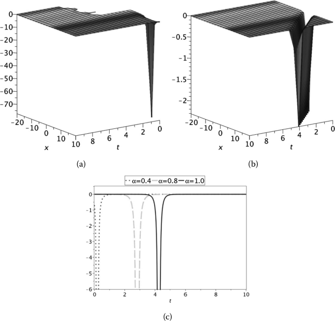
  Singular soliton solution of $u_{1,2} ( \xi )$

  Figure 3

  

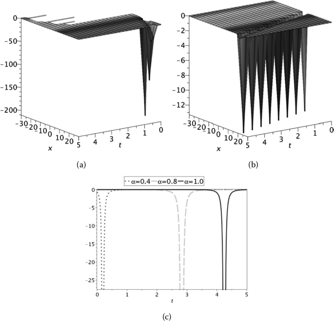
  Singular soliton solution of $u_{1,5} ( \xi )$

  Figure 4

  

  Bell type soliton solution of $u_{1,6} ( \xi )$

  Figure 5

  

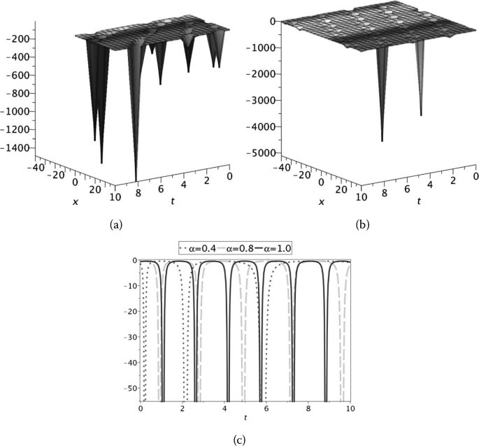
  Periodic solution of $u_{1,13} ( \xi )$

  Figure 6

  

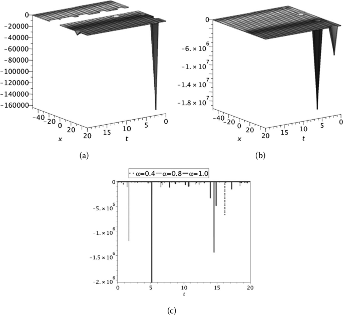
  Periodic solution of $u_{1,17} ( \xi )$

  Figure 7

  

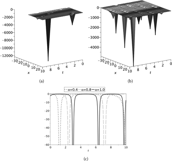
  Periodic solution of $u_{1,18} ( \xi )$

  Figure 8

  

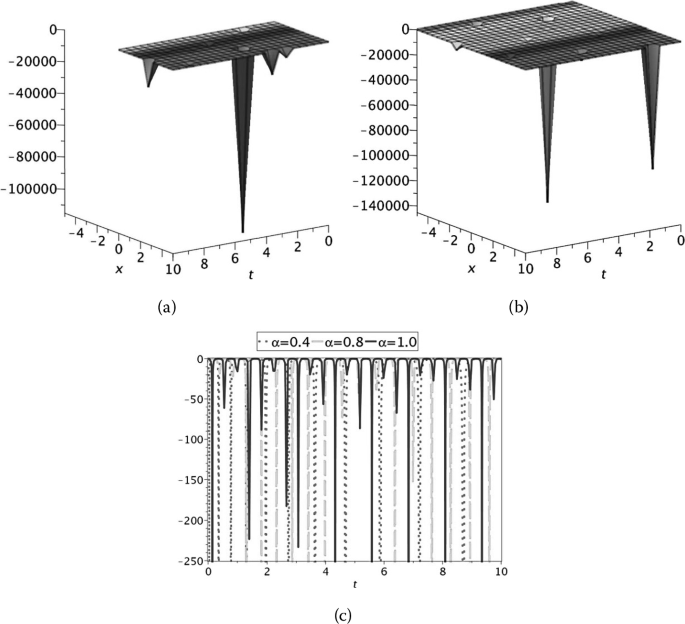
  Periodic solution of $u_{1,19} ( \xi )$

• II. Fig. 9 shows the graphical representation of a bell type soliton solution of $u_{2,1} ( \xi )$ with $p=4$, $q=2$, $r=1$, $\chi =0.3$ for $-5\leq x\leq 5$, $0\leq t<30$. The solution $u_{2,2} ( \xi )$ depicts the properties of a singular soliton solution of Eq. (40) with $p=3$, $q=1$, $r=1$, $\chi =0.5$ which are graphed in Fig. 10. Figure 11 represents the solitary wave solution of $u_{2,4} ( \xi )$ by considering $p=5$, $q=0.25$, $r=0.5$, $\chi =0.2$ within the interval $-10\leq x\leq 10$, $0\leq t<10$. The hyperbolic solution of Eq. (45) with $p=3$, $q=0.5$, $r=2$, $\chi =0.5$, $A=2$, $B=5$ for $-20\leq x\leq 20$, $0\leq t<10$ is depicted in Fig. 12. The trigonometric solution of $u_{2,13} ( \xi )$ and $u_{2,19} ( \xi )$ with $p=1$, $q=3$, $r=2$, $\chi =0.2$ for $-30\leq x\leq 30$, $0\leq t<50$ and $p=3$, $q=4$, $r=2$, $\chi =0.5$, $A=5$, $B=2$ for $-10\leq x\leq 10$, $0\leq t<5$, respectively.

  Figure 9

  

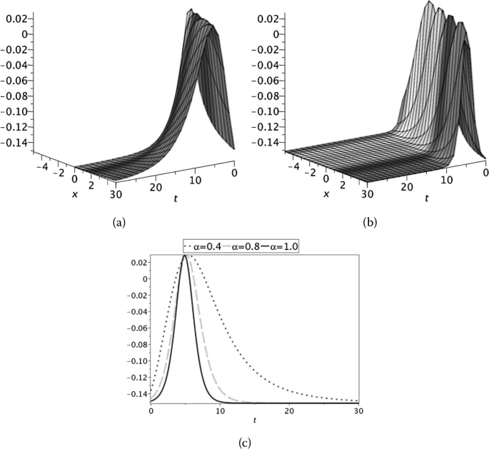
  Bell type soliton solution of $u_{2,1} ( \xi )$

  Figure 10

  

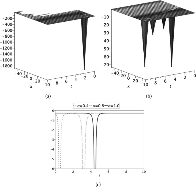
  Singular soliton solution of $u_{2,2} ( \xi )$

  Figure 11

  

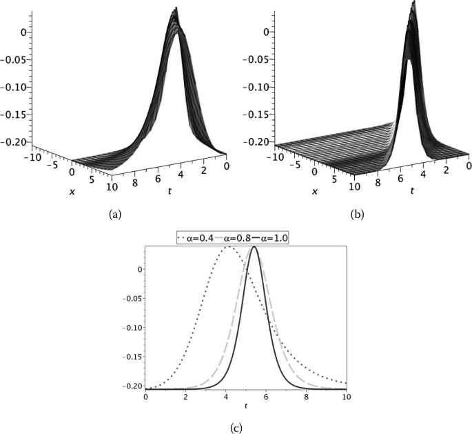
  Solitary wave solution of $u_{2,4} ( \xi )$

  Figure 12

  

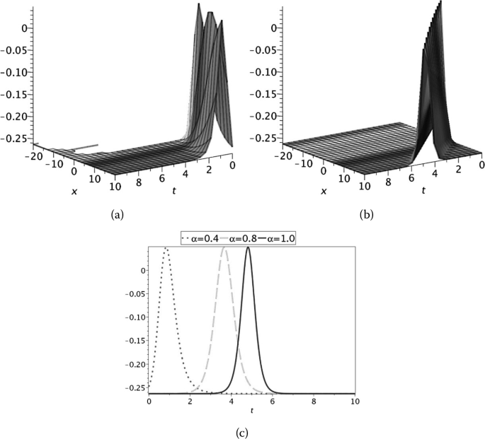
  Hyperbolic solution of $u_{2,7} ( \xi )$

  Figure 13

  

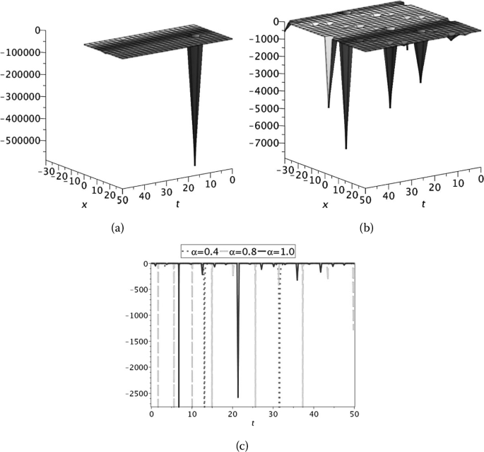
  Trignometric solution of $u_{2,13} ( \xi )$

  Figure 14

  

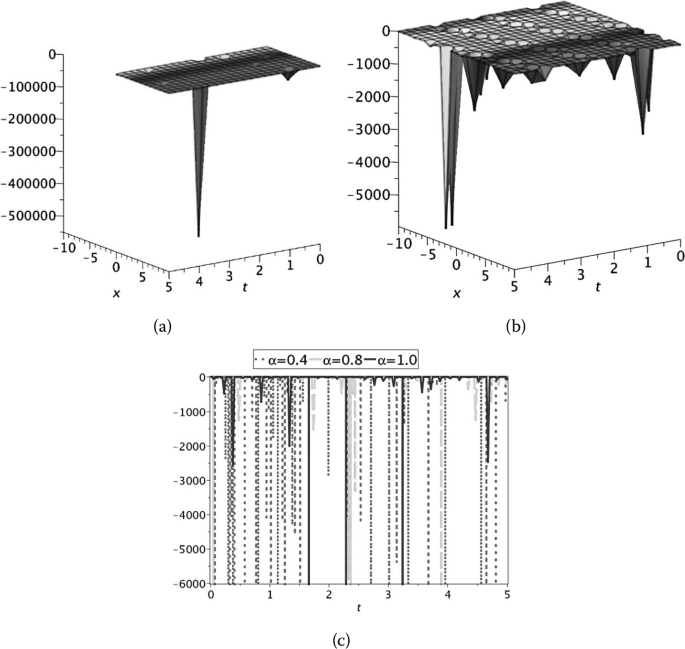
  Trignometric solution of $u_{2,19} ( \xi )$

5 Comparison of the obtained solutions

In this section, we discuss and make a comparison of the exact solutions. We will find the relationship between the exact solutions obtained by the generalized Riccati equation mapping method with Atangana–Baleanu fractional derivative applied on (CDG) equation and the exact solutions obtained by other methods. To the best of our knowledge, these exact solutions are new and not available in the literature. The tanh-coth [50] method was applied to investigate the fifth order Caudrey–Dodd–Gibbon equation and find out only four solutions. Neamaty et al. [51] executed the $( \frac{G '}{G} )$-expansion method and obtained only five travelling wave solutions. Yaslan et al. [52] investigated the same equation through the $( \frac{G '}{G^{2}} )$-expansion method and obtained only six solutions. The obtained solutions are expressed by hyperbolic, trigonometric, and rational solutions. However, we have attained twenty-seven travelling wave solutions by applying the generalized Riccati equation mapping method with Atangana–Baleanu fractional derivative. The obtained solutions might be useful to analyze the physical significance. Furthermore, for the definite values of the parameters, diverse known solitons, such as soliton, singular soliton, periodic, bell type, and dark solutions, are originated. Therefore, we might conclude that our obtained results are more general than those attained by other methods.

6 Conclusion

Generalized Riccati equation mapping approach is used to obtain periodic, hyperbolic, and rational solutions of space–time conformable Caudrey–Dodd–Gibbon (CDG) equation. These solutions include solitary wave solutions, which are dark, singular, and bell type soliton solutions, for suitable values of parameters. Our work (not reported yet in the literature) successfully finds solutions by using the conformable derivative. All the solutions are verified with the help of Maple 16. 2D and 3D graphical representations of some solutions are illustrated for the fractional orders $\alpha =0.4,0.8,1$ and $\alpha =0.4,1$, respectively. This method can be very promising for nonlinear equations and their systems in the study of mathematical physics.

References

1. Podlubny, I.: Fractional Differential Equations: An Introduction to Fractional Derivatives, Fractional Differential Equations, to Methods of Their Solution and Some of Their Applications (1998)
MATH  Google Scholar
2. Petráš, I.: Fractional-Order Nonlinear Systems: Modeling, Analysis and Simulation (2011)
3. Kumar, D., Singh, J., Baleanu, D., Rathore, S.: Analysis of a fractional model of the Ambartsumian equation. Eur. Phys. J. Plus 133(7), 259 (2018)
Google Scholar
4. Singh, J., Kumar, D., Baleanu, D., Rathore, S.: An efficient numerical algorithm for the fractional Drinfeld–Sokolov–Wilson equation. Appl. Math. Comput. 335, 12–24 (2018)
MathSciNet  Google Scholar
5. Kumar, D., Agarwal, R.P., Singh, J.: A modified numerical scheme and convergence analysis for fractional model of Lienard’s equation. J. Comput. Appl. Math. 339, 405–413 (2018)
MathSciNet  MATH  Google Scholar
6. Rashidi, M.M.: Corrigendum to ‘The modified differential transform method for solving MHD boundary-layer equations’ [Comput. Phys. Comm. 180 (2009) 2210–2217]. Comput. Phys. Commun. 212, 285 (2017)
7. Li, S., He, Y., Long, Y.: Joint application of bilinear operator and F-expansion method for \((2+1)\)-dimensional Kadomtsev–Petviashvili equation. Math. Probl. Eng. 2014, 1–5 (2014)
8. Eslami, M., Rezazadeh, H.: The first integral method for Wu–Zhang system with conformable time-fractional derivative. Calcolo 53(3), 475–485 (2016)
9. Feng, D., Li, K.: Exact traveling wave solutions for a generalized Hirota–Satsuma coupled KdV equation by Fan sub-equation method. Phys. Lett. A 375(23), 2201–2210 (2011)
10. Mirzazadeh, M., Eslami, M., Zerrad, E., Mahmood, M.F., Biswas, A., Belic, M.: Optical solitons in nonlinear directional couplers by sine–cosine function method and Bernoulli’s equation approach. Nonlinear Dyn. 81(4), 1933–1949 (2015)
11. He, J.H., Wu, X.H.: Construction of solitary solution and compacton-like solution by variational iteration method. Chaos Solitons Fractals 29(1), 108–113 (2006)
12. Mohyud-Din, S.T., Noor, M.A., Noor, K.I., Hosseini, M.M.: Variational iteration method for re-formulated partial differential equations. Int. J. Nonlinear Sci. Numer. Simul. 11(2), 87–92 (2010)
13. Mohyud-Din, S.T., Bibi, S.: Exact solutions for nonlinear fractional differential equations using exponential rational function method. Opt. Quantum Electron. 49(2), 64 (2017)
14. Mohyud-Din, S.T., Bibi, S., Ahmed, N., Khan, U.: Some exact solutions of the nonlinear space–time fractional differential equations. Waves Random Complex Media (2018). https://doi.org/10.1080/17455030.2018.1462541
15. Wu, X.H.B., He, J.H.: Solitary solutions, periodic solutions and compacton-like solutions using the Exp-function method. Comput. Math. Appl. 54(7–8), 966–986 (2007)
16. Mohyud-Din, S.T., Khan, Y., Faraz, N., Yıldırım, A.: Exp-function method for solitary and periodic solutions of Fitzhugh–Nagumo equation. Int. J. Numer. Methods Heat Fluid Flow 22(3), 335–341 (2012)
17. Wu, X.-H.B., He, J.-H.: EXP-function method and its application to nonlinear equations. Chaos Solitons Fractals 38(3), 903–910 (2008)
18. He, J.-H., Wu, X.-H.: Exp-function method for nonlinear wave equations. Chaos Solitons Fractals 30(3), 700–708 (2006)
19. Teymuri Sindi, C., Manafian, J.: Wave solutions for variants of the KdV–Burger and the \(K(n,n)\)-Burger equations by the generalized \(G'/G\)-expansion method. Math. Methods Appl. Sci. 40(12), 4350–4363 (2017)
20. Sindi, C.T., Manafian, J.: Soliton solutions of the quantum Zakharov–Kuznetsov equation which arises in quantum magneto-plasmas. Eur. Phys. J. Plus 132(2), 67 (2017)
21. Manafian, J., Aghdaei, M.F., Khalilian, M., Sarbaz Jeddi, R.: Application of the generalized \(G'/G\)-expansion method for nonlinear PDEs to obtaining soliton wave solution. Optik 135, 395–406 (2017)
22. Roshid, H.-O., Kabir, M., Bhowmik, R., Datta, B.: Investigation of solitary wave solutions for Vakhnenko–Parkes equation via exp-function and \(\mathit{Exp}(- \phi (\xi ))\)-expansion method. SpringerPlus 3(1), 692 (2014)
23. Aghdaei, M.F., Manafian, J.: Optical soliton wave solutions to the resonant Davey–Stewartson system. Opt. Quantum Electron. 48, 413 (2016)
24. Inan, I.E., Duran, S., Uğurlu, Y.: \(\mathit{TAN}(F(\xi /2))\)-Expansion method for traveling wave solutions of AKNS and Burgers-like equations. Optik 138, 15–20 (2017)
25. Bulut, H., Pandir, Y.: Modified trial equation method to the nonlinear fractional Sharma–Tasso–Olever equation. Int. J. Model. Optim. 3(4), 353–357 (2013)
26. Odabasi, M., Misirli, E.: On the solutions of the nonlinear fractional differential equations via the modified trial equation method. Math. Methods Appl. Sci. 41(3), 904–911 (2018)
27. Baleanu, D., Jajarmi, A., Hajipour, M.: On the nonlinear dynamical systems within the generalized fractional derivatives with Mittag-Leffler kernel. Nonlinear Dyn. 94(1), 397–414 (2018)
28. Jajarmi, A., Baleanu, D.: A new fractional analysis on the interaction of HIV with CD4+ T-cells. Chaos Solitons Fractals 113, 221–229 (2018)
29. Baleanu, D., Jajarmi, A., Bonyah, E., Hajipour, M.: New aspects of poor nutrition in the life cycle within the fractional calculus. Adv. Differ. Equ. 2018(1), 230 (2018)
30. Jajarmi, A., Baleanu, D.: Suboptimal control of fractional-order dynamic systems with delay argument. J. Vib. Control 24(12), 2430–2446 (2018)
31. Kumar, D., Singh, J., Baleanu, D.: A new analysis of the Fornberg–Whitham equation pertaining to a fractional derivative with Mittag-Leffler-type kernel. Eur. Phys. J. Plus 133(2), 70 (2018)
32. Singh, J., Kumar, D., Hammouch, Z., Atangana, A.: A fractional epidemiological model for computer viruses pertaining to a new fractional derivative. Appl. Math. Comput. 316, 504–515 (2018)
33. Khalil, R., Al Horani, M., Yousef, A., Sababheh, M.: A new definition of fractional derivative. J. Comput. Appl. Math. 264, 65–70 (2014)
34. Atangana, A., Baleanu, D., Alsaedi, A.: New properties of conformable derivative. Open Math. 13(1), 889–898 (2015)
35. Çenesiz, Y., Baleanu, D., Kurt, A., Tasbozan, O.: New exact solutions of Burgers’ type equations with conformable derivative. Waves Random Complex Media 27(1), 103–116 (2017)
36. He, S., Sun, K., Mei, X., Yan, B., Xu, S.: Numerical analysis of a fractional-order chaotic system based on conformable fractional-order derivative. Eur. Phys. J. Plus 132(1), 36 (2017)
37. Rezazadeh, H., Pourreza Ziabary, B.: Sub-equation method for the conformable fractional generalized Kuramoto–Sivashinsky equation. Comput. Res. Prog. Appl. Sci. Eng. 2(3), 106–109 (2016)
38. Aminikhah, H., Sheikhani, A.H.R., Rezazadeh, H.: Sub-equation method for the fractional regularized long-wave equations with conformable fractional derivatives. Sci. Iran. 23(3), 1048–1054 (2016)
39. Hosseini, K., Ansari, R.: New exact solutions of nonlinear conformable time-fractional Boussinesq equations using the modified Kudryashov method. Waves Random Complex Media 27(4), 628–636 (2017)
40. Cenesiz, Y., Tasbozan, O., Kurt, A.: Functional Variable Method for conformable fractional modified KdV–ZK equation and Maccari system. Tbil. Math. J. 10(1), 117–125 (2017)
41. Atangana, A., Baleanu, D., Alsaedi, A.: Analysis of time-fractional Hunter–Saxton equation: a model of neumatic liquid crystal. Open Phys. 14(1), 145–149 (2016)
42. Atangana, A., Baleanu, D.: New fractional derivatives with non-local and non-singular kernel. Therm. Sci. 20(2), 763–769 (2016)
43. Wazwaz, A.-M.: Analytic study of the fifth order integrable nonlinear evolution equations by using the tanh method. Appl. Math. Comput. 174(1), 289–299 (2006)
44. Xu, Y.G., Zhou, X.W., Yao, L.: Solving the fifth order Caudrey–Dodd–Gibbon (CDG) equation using the exp-function method. Appl. Math. Comput. 206(1), 70–73 (2008)
45. Naher, H., Abdullah, F.A., Akbar, M.A.: The \((G'/G)\)-expansion method for abundant traveling wave solutions of Caudrey–Dodd–Gibbon equation. Math. Probl. Eng. 2011, 1–11 (2011)
46. Elsayed, M.E.Z., Yasser, A.A., Reham, M.A.S.: The improved generalized Riccati equation mapping method and its application for solving a nonlinear partial differential equation (PDE) describing the dynamics of ionic currents along microtubules. Sci. Res. Essays 9(8), 238–248 (2014)
47. Zayed, E.M.E., Al-Nowehy, A.-G.: Solitons and other solutions to the nonlinear Bogoyavlenskii equations using the generalized Riccati equation mapping method. Opt. Quantum Electron. 49(11), 359 (2017)
48. Malwe, B.H., Betchewe, G., Doka, S.Y., Kofane, T.C.: Travelling wave solutions and soliton solutions for the nonlinear transmission line using the generalized Riccati equation mapping method. Nonlinear Dyn. 84(1), 171–177 (2016)
49. Zhu, S.: The generalizing Riccati equation mapping method in non-linear evolution equation: application to \((2+1)\)-dimensional Boiti–Leon–Pempinelle equation. Chaos Solitons Fractals 37(5), 1335–1342 (2008)
50. Wazwaz, A.M.: Multiple-soliton solutions for the fifth order Caudrey–Dodd–Gibbon (CDG) equation. Appl. Math. Comput. 197(2), 719–724 (2008)
51. Neamaty, A., Agheli, B., Darzi, R.: Exact travelling wave solutions for some nonlinear time fractional fifth-order Caudrey–Dodd–Gibbon equation by \(( G'/G)\)-expansion method. SeMA J. 73(2), 121–129 (2016)
52. Yaslan, H.C., Girgin, A.: New exact solutions for the conformable space–time fractional KdV, CDG, \((2+1)\)-dimensional CBS and \((2+1)\)-dimensional AKNS equations. J. Taibah Univ. Sci. 13(1), 1–8 (2019)
Download references
Acknowledgements
Authors are grateful to the anonymous reviewers for useful comments that helped in improving the quality of manuscript.
Funding
Authors received no funding for the research.
Author information
Authors and Affiliations
Authors
Contributions
All authors drafted the manuscript, and they read and approved the final version of the manuscript.
Corresponding author
Correspondence to Imran Faisal.
Ethics declarations
Competing interests
Authors declare that they have no competing interests.
Additional information
Publisher’s Note
Springer Nature remains neutral with regard to jurisdictional claims in published maps and institutional affiliations.
Rights and permissions
Open Access This article is distributed under the terms of the Creative Commons Attribution 4.0 International License (http://creativecommons.org/licenses/by/4.0/), which permits unrestricted use, distribution, and reproduction in any medium, provided you give appropriate credit to the original author(s) and the source, provide a link to the Creative Commons license, and indicate if changes were made.
Reprints and permissions
About this article
Check for updates. Verify currency and authenticity via CrossMark
Cite this article
Bibi, S., Ahmed, N., Faisal, I. et al. Some new solutions of the Caudrey–Dodd–Gibbon (CDG) equation using the conformable derivative. Adv Differ Equ 2019, 89 (2019). https://doi.org/10.1186/s13662-019-2030-7
Download citation
• Received:
• Accepted:
• Published:
• DOI: https://doi.org/10.1186/s13662-019-2030-7