A switched multicontroller for an SEIADR epidemic model with monitored equilibrium points and supervised transients and vaccination costs

Abstract

This paper presents a multicontroller structure for an SEIADR (susceptible-exposed-symptomatic infectious-asymptomatic infectious-dead lying bodies recovered by immunity, or immune, subpopulations) epidemic model, which has three different controls involving feedback, namely, the vaccination on the susceptible subpopulation, the antiviral treatment on the symptomatic infectious subpopulation, and the impulsive removal on the infective lying bodies. The incorporation of the asymptomatic infectious and infective dead bodies to SEIR-type models allows a better modeling of diseases where the death bodies are infective as, for instance, the Ebola disease. The proposed supervised multicontroller scheme consists of a parallel disposal of several alternative controller parameterizations together with a switching scheme that chooses the active controller through consecutive time intervals via a supervisory decision scheme. The supervisory scheme decides to switch or not at testing time instants. Switching is performed to a distinct active scheme to the current active if the tentative controller minimizes the value of a loss function compared to the values of the other control schemes available in the parallel controller disposal. The supervisory loss (or cost) function incorporates several additive weighted terms including the infection loss function evolution and the vaccination, antiviral treatment, and bodies removal efforts.

1 Introduction

Relevant attention is being paid in the last two decades to the study of mathematical epidemic models that are modeled by integro-differential equations and/or difference equations. Those models describe the evolution of various considered subpopulations as the disease under study progresses. Typically, the models have three essential subpopulations (namely, susceptible, infectious, and recovered by immunity) whose dynamics are mutually coupled. There are different degrees of complexity in the statement of the models. The simplest ones have only “susceptible” (S) and “infectious” (I) subpopulations and are referred to as SI-models. A second degree of complexity adds a third one said to be the “recovered by immunity” subpopulation, and those models are said to be SIR-models. A further complexity degree splits the infectious into two subpopulations (or compartments), namely, the so-called “infected” or “exposed” (E) (those having the disease but do not present yet external symptoms) and the “infectious” or “infective” (those having external symptoms). The generic acronym used for this last category of models is SEIR, referred to as SEIR epidemic models. General description of epidemic models and some mathematical analysis on them is given in some classical books. See, for instance, [1–3]. Specific models for Ebola, which is the infection of major interest for the formulation of this paper, are recently discussed in [4–6]. For alternative epidemic models, see, for instance, [7–9]. In particular, a homotopy analysis is developed in [8], and a pulse vaccination rule is suggested and discussed in [9] and some references therein. The positivity of the solution is investigated in a number of works. See, for instance, [10–13] and [14] and some references therein. In particular, the properties of boundedness, oscillatory behaviors, positivity, and stability together with the injection of some constant, feedback regular, and impulsive control laws are investigated in [10, 11] in proposed true-mass epidemic SEIR models with uncertainties and eventual delays. Very general vaccination rules are studied more in detail in [12], whereas distributed delays in the epidemic model are introduced in [13]. Also, certain robustness studies of stability and positivity under deviations of the equilibrium points due to Wiener noise are performed in [13]. In particular, the regular feedback laws can involve control gains to consider proportionality to one of more subpopulations, whereas the impulsive ones can also have feedback information. The use of nonlinear incidence rates in the models is also investigated in a number of papers. See, for instance, [15–17]. The rules for discretization and the presence of perturbations are also investigated in many epidemic models. See, for instance, [17–21], some of them being formulated in a stochastic framework. In particular, in [17] the incidence rate is assumed to be saturated, whereas the random perturbations fluctuate. Also, a nonstandard discretization of epidemic models is proposed in [18], whereas the global asymptotic stability to the equilibrium under incidence rate of saturated mass action and feedback controls is investigated in [19]. In [20], sufficient conditions for the stability in probability of the equilibrium states are derived for a Nowak–May-type model. On the other hand, exponential nonlinearities are introduced in the stochastic epidemic model of [21].

The stability properties and the convergence of the solutions to the equilibrium states are major analysis tools in most of the works. In particular, the asymptotic solution behaviors including associated diffusion effects have been provided in [22, 23] and some references therein. More work on the use of vaccination rules to improve the infection behavior through time has been proposed in the background literature. See, for instance, [24–27] and some references therein. In particular, two control actions are proposed in [24], namely, a vaccination action on the susceptible subpopulation and a therapeutic treatment on the infectious subpopulation with constant and nonconstant controls and impulsive controls are proposed in [26–28]. The stability and optimal control under a subpopulation of infective individuals in treatment with vaccination is investigated in [29], and a model with delay, latent period, and saturation incidence rate and impulsive vaccination is proposed and discussed in [30].

On the other hand, it turns out that, as it is known due to medical experience, there are individuals who are infective but do not have significant external symptoms, that is, the so-called the “asymptomatic” (A) subpopulation [7] can be present in the illness evolution. This feature occurs even in the common known influenza disease. If such an asymptomatic subpopulation is considered in the model, then it turns out that the exposed have different transitions to the symptomatic infectious and to the asymptomatic ones so that a part of the exposed become asymptomatic infectious after a certain time while others become symptomatic infectious. Finally, it is well known that in the case of Ebola disease, the infective lying dead corpses are infective [4–7], which causes serious sanitary problems in third-world tropical countries with low or scarce sanitary means when an Ebola disease spreads thoroughly, especially when it is transmitted from rural areas to high-populated urban ones. The dead infective corpses can be considered in the model as a new subpopulation “D”.

It is well known from the related background literature that a parallel disposal of multiestimation or multicontrol devices (or hybrid of both of them), together with a supervisory scheme for switching through time for choosing the active scheme, can improve very much the transient performance. Another advantage is that, due to the parallel computational structure, the multicontroller-supervised scheme is not excessively time consuming compared to the use of a single-controller. Basically, the computation time on an active interval is that associated with a single controller plus the moderate calculation time of the supervisory decision about the next switching action. Such a performance is evaluated in terms of minimizing a judiciously defined loss function being a measure of the current system behavior or, eventually, of the discrepancies compared to the suited ideal behavior if available. The online supervisory action decides if the active configuration has to be switched or not at each current tentative testing switching time instant. See, for instance, [14, 31–33], references therein, and [34]. In particular, the parametrical estimation is incorporated as well in [35–38] to identify potentially unknown system parameters. It can be pointed out that supervision, or monitoring, techniques are very common as strategies to improve the performances in a wide variety of problems like, for instance, in problems of updating sampling rates in data acquisition according to the sampled signal dominant frequencies, in multirate sampling problems associated with the need for using different sampling periods for distinct signals integrated in the same problem to deal with, in classification techniques in random fields or the supervision of time intervals for the activation of devices in machine-to-machine communication problems, etc. See, for instance, [31–33] and also [37–40] related to the two last mentioned potential applications. The main objective of this paper is to develop a parallel multicontroller scheme with a supervisory scheme for the online decision on the choice of the appropriate active configuration. The number of models of the parallel structure can be either constant through time or, eventually, time-varying while constant in each interswitching time interval. The supervision scheme decides on each current active controller by choosing the one that minimizes its supervisory loss function. Several variants of the design strategies to follow are proposed and discussed. In particular, the decision time instant candidates can be anyone satisfying a minimum permanence threshold interval at each active configuration or multiple of a “minimum residence” (or “dwelling”) time interval compatible with the stability properties. On the other hand, the loss functions to decide on switching or not to the next active configuration can have several weighted additive terms of free-design choice, typically, the infection cost evolution and the vaccination/treatment/corpses removal costs. Also, the strategies can have the objective of targeting a prescribed stable disease-free equilibrium solutions in the case this objective is feasible or to reject approaching to the endemic equilibrium solution, if this one is stable, by conducting the trajectory solution to oscillate around both equilibrium solutions. Alternatively, the disease-free solution for the nonzero components (i.e. susceptible and recovered subpopulations) can be allowed to be of free-design as the best supervisory function evolves with time. On the other hand, it is also possible the use of distinct time-invariant model parameterizations, each one with an associate parallel multicontroller scheme. This strategy can be useful, in particular, when the model is uncertain around a nominal parameterization so that the control multischeme can include tandems of model parameterizations, each with a set of associated controllers in a parallel disposal. It can be pointed out that the proposed supervisory scheme can be a simple alternative to the use of optimal control techniques, which are difficult to rigorously apply due to the highly nonlinear nature of the problem at hand. On the other hand, the importance of the discretization of mathematical models is relevant in certain practical real problems. For instance, some coupled difference equations and the associated convergence problems have been studied in [41], whereas the estimation of parameters of epidemic models has been dealt with in [42]. In this work, the switched mechanism is deliberately introduced to improve the controlled behavior of the evolution of the epidemic. In this way, the approach adopted in this paper is definitely different from previous ones. Another novelty is the incorporation of the dead-infective subpopulation and the culling action, interpreted as an impulsive control on the subpopulation time-derivative. Performed simulation examples show the usefulness of the proposed supervision for the Ebola spread.

The paper is organized as follows. Section 2 introduces the SEIADR model with six subpopulations (S, E, I, A, D, R) under controls in terms of vaccination control on the susceptible and antiviral treatment on the symptomatic infectious subpopulation. Such controls are combinations of feedback-independent (which can be constant, in particular) and feedback-linear terms. There is also an additional impulsive control action of retirement of corpses to reduce the risks of dead-contagion to the alive uninfectious population. The controls can have feedback information taken on line from their respective subpopulations and are not exerted necessarily at the same impulsive time instants. Section 3 summarizes some local and global stability conditions proved in the background literature together with some further direct conclusion about the variation of the nonzero-component disease-free equilibrium points depending on the limit vaccination gains. The disease-free equilibrium point is specified, and some concerns about the existence of endemic equilibrium solutions (which can be, in particular, endemic equilibrium points) are given in terms of the size of the coefficient transmission rates being below certain threshold value. Section 4 describes and develops the parallel multicontroller scheme with different optional variants to define and address the losses functions that measure with predesigned or updated weighting terms the infection and vaccination costs. In particular, the switching time instants for the decision on the next active configuration in operation can be multiple of a minimum constant threshold interval or time-varying when evaluating the supervisory losses function of each testable control configuration. The parameterizations of the multicontrol scheme can be either prefixed through time or of updated values at each new switching time instant around each active one in operation. Also, the scheme can be adapted to uncertain or time-varying models under certain a priori knowledge of the parameterizations by using tandems of parallel multicontrol schemes for distinct constant parameterizations around a nominal time-invariant one. Section 5 gives and discusses some numerical comparative examples and emphasizes the advantages of the use of parallel controller disposals against the use of fixed ones, especially, in the cases of uncertain or time-varying models or when a low vaccination cost or infection evolution through time is suited. Finally, conclusions end the paper.

1.1 Notation

$$\begin{aligned}& \boldsymbol{R}_{ +} = \{ r \in \boldsymbol{R}: r > 0 \},\qquad \boldsymbol{R}_{0 +} = \{ r \in \boldsymbol{R}: r \ge 0 \}, \\& \boldsymbol{Z}_{ +} = \{ r \in \boldsymbol{Z}: r > 0 \},\qquad \boldsymbol{Z}_{0 +} = \{ r \in \boldsymbol{Z}: r \ge 0 \}. \end{aligned}$$

The symbols ∨ and ∧ stand, respectively, for logic “or” and “and”.

$C^{0}$ and $PC^{0}$ are, respectively, the sets of continuous and piecewise continuous functions on domain I with image X. The functions $f:I \to X$ in those sets are denoted, respectively, by $f \in C^{0} ( I, X )$ and $f \in PC^{0} ( I, X )$.

$\operatorname{card} ( A )$ denotes the cardinality of a set A, $\operatorname{card} ( A ) = \aleph_{0}$ indicates that the cardinality of a denumerable set A is infinity as opposed to $\operatorname{card} ( A ) = \infty$, denoting the infinite cardinality of a nondenumerable set A.

$\boldsymbol{I}_{n}$ is the nth identity matrix, $\delta ( t )$ denotes the Dirac distribution at $t = 0$, $\overline{m} = \{ 1, 2,\ldots, m \}$.

2 The SEIADR epidemic model

An SEIADR model is an extended SEIR model proposed in [43]. Apart from the classical subpopulations of “susceptible” (S), “exposed” (E), “symptomatic infectious” (I), and “recovered” (or immune) (R), it has two additional subpopulations, namely, “asymptomatic infectious” (A) and “dead-infective” (D). It can be of interest for certain infective diseases for which the lying bodies are extra infective subpopulations, for instance, in the case of Ebola. This model incorporates three controls, which can be combined to define the whole control to be injected. Those controls are the vaccination control on the susceptible subpopulation, the antiviral treatment on the infective subpopulation, and the dead-infective removal. The epidemic SEIADR model is the following one:

$$\begin{aligned}& \dot{S} ( t ) = b_{1} - \bigl( b_{2} + \beta I ( t ) + \beta_{A}A ( t ) + \beta_{D} D ( t ) \bigr) S ( t ) + \eta R ( t ) - V ( t ), \end{aligned}$$

(1)

$$\begin{aligned}& \dot{E} ( t ) = - ( b_{2} + \gamma ) E ( t ) + \bigl( \beta I ( t ) + \beta_{A}A ( t ) + \beta_{D} D ( t ) \bigr) S ( t ), \end{aligned}$$

(2)

$$\begin{aligned}& \dot{I} ( t ) = - ( b_{2} + \alpha + \tau_{0} ) I ( t ) + \gamma p E ( t ) - \xi ( t ), \end{aligned}$$

(3)

$$\begin{aligned}& \dot{A} ( t ) = - ( b_{2} + \tau_{0} ) A ( t ) + \gamma ( 1 - p ) E ( t ), \end{aligned}$$

(4)

$$\begin{aligned}& \dot{D} ( t ) = - \mu D ( t ) + b_{2} \bigl( I ( t ) + A ( t ) \bigr) + \alpha I ( t ) - \theta ( t ), \end{aligned}$$

(5)

$$\begin{aligned}& \dot{R} ( t ) = - ( b_{2} + \eta ) R ( t ) + \tau_{0} \bigl( I ( t ) + A ( t ) \bigr) + \xi ( t ) + V ( t ), \end{aligned}$$

(6)

$$\begin{aligned}& V ( t ) = V_{0} ( t ) + K_{V} ( t )S ( t ), \end{aligned}$$

(7)

$$\begin{aligned}& \xi ( t ) = K_{\xi} ( t )I ( t ), \end{aligned}$$

(8)

$$\begin{aligned}& \theta ( t ) = \rho_{D} ( t ) D ( t ) \sum _{t_{\theta i} \in \operatorname{Imp}D} \delta ( t - t_{\theta i} ), \end{aligned}$$

(9)

for all $t\in R_{0+}$ with initial conditions satisfying $\min ( S ( 0 ), E ( 0 ), I ( 0 ), A ( 0 ), D ( 0 ), R ( 0 ) ) \ge 0$, where:

$$\operatorname{Imp}D = \bigl\{ t \in \boldsymbol{R}_{0 +} : D ( t ) \ne D \bigl( t^{ -} \bigr) \bigr\} = \bigcup_{t \in \boldsymbol{R}_{0 +}} \operatorname{Imp}D ( t ) $$

is the total set of impulsive (“removal”) time instants $t_{\theta i} \in \operatorname{Imp}D$ for removal of infective corpses (note that the notation for $f ( t^{ +} )$ is simplified to $f ( t )$). Besides,

$$\begin{aligned}& \operatorname{Imp}D \bigl( t^{ -} \bigr) = \{ \sigma \in \operatorname{Imp}D : \sigma < t \}, \\& \operatorname{Imp}D ( t ) = \{ \sigma \in \operatorname{Imp}D : \sigma \le t \} = \operatorname{Imp}D \bigl( t^{ -} \bigr)\quad \mbox{if } t \notin \operatorname{Imp}D,\quad \mbox{and} \\& \operatorname{Imp}D ( t ) = \{ \sigma \in \operatorname{Imp}D : \sigma \le t \} = \operatorname{Imp}D \bigl( t^{ -} \bigr) \cup \{ t \}\quad \mbox{if } t \in \operatorname{Imp}D, \end{aligned}$$

and the (nonnegative) parameters and controls are the following ones:

• $b_{1}$ is the recruitment rate,

• $b_{2}$ is the natural average death rate,

• β, $\beta_{A}$, $\beta_{D}$ are the various disease transmission coefficients from the susceptible to the respective symptomatic infectious, asymptomatic, and infective corpses subpopulations,

• η is a parameter such that $1/\eta$ is the average duration of the immunity period reflecting a transition from the recovered to the susceptible,

• γ is the transition rate from the exposed to all (i.e. both symptomatic and asymptomatic) infectious,

• α is the average extra mortality associated with the symptomatic infectious subpopulation,

• $\tau_{0}$ is the natural immune response rate for the whole infectious subpopulation (i.e. $A + I$), respectively, p is the fraction of the exposed individuals that become symptomatic infectious,

• $1 - p$ is the fraction of the exposed that become asymptomatic infectious,

• $1/\mu$ is the average period of infectiousness after death,

• $V ( t )$ and $\xi ( t )$ are, respectively, the vaccination and antiviral treatment controls, and $\rho_{D} ( t_{\theta i} ) D ( t_{\theta i} )$ is the impulsive action of removal of corpses (or “removal”) for all $t_{\theta i} \in \operatorname{Imp}D$ with $\rho_{D} ( t ) \in [ 0, 1 ]$.

The above model has the subsequent basic characteristics:

• (a) It is assumed that the mortality rate of the asymptomatic subpopulation is similar to that of the healthy one. Thus, there is no extra disease mortality associated with the asymptomatic infectious subpopulation, whereas there is an extra mortality rate associated with the symptomatic infectious subpopulation.

• (b) The model lies into the class of pseudo-mass action (or density-dependent) class of epidemic models. Those models are not subject to disease transmission rates modulated by the total population. It is well known that there is another class of models, the so-called true-mass (or frequency-dependent) epidemic models. In these models, the transmission rates are normalized by the total population, and the simple physical interpretation is that the contagion rates decrease as the environment total population increases [44].

• (c) The controls (7)–(9) can be of different types including constant and feedback actions. The nonnegativity and boundedness of the solutions through time, the equilibrium points, their stability, and the existence of eventual limit oscillatory solutions and their stability properties have been investigated in [43]. The study of those properties is common in a wide sampling of other alternative epidemic models discussed in the background literature. See, for instance, [10–16, 22, 23], and [45, 46]. In particular, a discrete epidemic model is investigated in [14], which possesses a unique nonnegative equilibrium to which the solutions converge, and the case of imperfect vaccination under nonlinear incidence rate is investigated in [16]. On the other hand, in [47], general conditions for maintenance of the positivity of a dynamic system under its discretization are given and discussed. An illustrative flux diagram in the absence of vaccination, antiviral treatment, and corpses removal controls (7)–(9) is shown in Fig. 1. The transitions between various subpopulations of the model (white thick arrows) and their coupled dynamics (black thin arrows), defined by Eqs. (1)–(6), are also displayed.

  Figure 1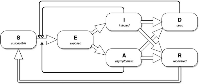

  

  Flow diagram of the control-free model transitions

3 SEIADR model, its equilibrium solutions and their stability properties

The following result holds concerning the disease-free equilibrium point.

Theorem 1

Assume that $V_{0} ( t ) \to V_{0}^{*}$, $K_{V} ( t ) \to K_{V}^{*}$, $K_{\xi} ( t ) \to K_{\xi}^{*}$ taking nonnegative values all the time and $\rho_{D} ( t_{\theta i} ) \to \rho_{D}^{*} = 0$ and $( t_{\theta ,i + 1} - t_{\theta i} ) \to T_{D}^{*}$ as $t, t_{\theta i}\ ( \in \operatorname{Imp}D ) \to \infty$. Assume also that $V_{0} ( t ) \in [ 0, b_{1} ]$, $\min ( K_{V} ( t ),K_{\xi} ( t ) ) \ge 0$, and $\rho_{D} ( t ) \in [ 0, 1 ]$ for all $t \in \boldsymbol{R}_{0 +}$. Then, all the subpopulations are nonnegative all the time under nonnegative initial conditions, and, furthermore, the following properties hold:

(i) (Theorem 5(i) of [43]). There is a unique disease-free equilibrium point satisfying

$$x_{\mathrm{df}}^{*}: = \lim_{t \to \infty} x ( t ) = \bigl( S_{\mathrm{df}}^{*} , E_{\mathrm{df}}^{*} , I_{\mathrm{df}}^{*} , A_{\mathrm{df}}^{*}, D_{\mathrm{df}}^{*} , R_{\mathrm{df}}^{*} \bigr) ^{T} = \bigl( S_{\mathrm{df}}^{*} , 0 , 0 , 0, 0 , R_{\mathrm{df}}^{*} \bigr) ^{T} $$

with

$$ S_{\mathrm{df}}^{*} = \frac{b_{2} ( b_{1} - V_{0}^{*} ) + \eta b_{1}}{b_{2} ( b_{2} + \eta + K_{V}^{*} )} = \frac{b_{1} + \eta N_{\mathrm{df}}^{*} - V_{0}^{*}}{b_{2} + \eta + K_{V}^{*}} $$

(10)

and

$$ R_{\mathrm{df}}^{*} = \frac{b_{2}V_{0}^{*} + K_{V}^{*}b_{1}}{b_{2} ( b_{2} + \eta + K_{V}^{*} )} = \frac{K_{V}^{*}N_{\mathrm{df}}^{*} + V_{0}^{*}}{b_{2} + \eta + K_{V}^{*}} = \frac{K_{V}^{*} S_{\mathrm{df}}^{*} + V_{0}^{*}}{b_{2} + \eta} = N_{\mathrm{df}}^{*} - S_{\mathrm{df}}^{*}, $$

(11)

leading to an associated limit total population $\overline{N}_{\mathrm{df}}^{*} = N_{\mathrm{df}}^{*} + D_{\mathrm{df}}^{*} = N_{\mathrm{df}}^{*} = S_{\mathrm{df}}^{*} + R_{\mathrm{df}}^{*} = \frac{b_{1}}{b_{2}}$ under a vaccination disease-free limit control $V_{\mathrm{df}}^{*} = V_{0}^{*} + K_{V}^{*}S_{\mathrm{df}}^{*}$ and a zero antiviral treatment limit control.

(ii) For any given real constant $\lambda \in [ 0, \frac{b_{2} + \eta}{b_{2} + \eta + K_{V}^{*}} ]$, the susceptible and immune equilibrium subpopulations can be prefixed to values $S_{\mathrm{df}}^{*} = \lambda N_{\mathrm{df}}^{*} = \lambda b_{1}/b_{2}$ and $R_{\mathrm{df}}^{*} = ( 1 - \lambda )N_{\mathrm{df}}^{*} = ( 1 - \lambda ) b_{1}/b_{2}$, respectively, by injecting a constant vaccination on the susceptible subpopulation given by

$$\begin{aligned} V_{0}^{*} &= V_{\mathrm{df}}^{*} - K_{V}^{*}S_{\mathrm{df}}^{*} = V_{\mathrm{df}}^{*} - \lambda K_{V}^{*} \frac{b_{1}}{b_{2}} \\ &= b_{1} \biggl[ 1 - \lambda + \frac{1}{b_{2}} \bigl( ( 1 - \lambda ) \eta - \lambda K_{V}^{*} \bigr) \biggr] \end{aligned}$$

or

$$K_{V}^{*} = \frac{1}{\lambda} \biggl[ \eta - \frac{b_{2}}{b_{1}} \bigl( V_{0}^{*} - b_{1} \bigr) \biggr] - b_{2} - \eta \quad \textit{if }\lambda \in ( 0, 1 ]. $$

In particular:

If $V_{0}^{*} = K_{V}^{*} = 0$ (vaccination-free case), then $S_{\mathrm{df}}^{*} = N_{\mathrm{df}}^{*} = b_{1}/b_{2}$ and $R_{\mathrm{df}}^{*} = 0$ with $\lambda = 1$.

If $K_{V}^{*} = b_{2} + \eta$ and $V_{0}^{*} = 0$, then $S_{\mathrm{df}}^{*} = R_{\mathrm{df}}^{*} = N_{\mathrm{df}}^{*}/2 = \frac{b_{1}}{2b_{2}}$ with $\lambda = 1/2$.

If $V_{0}^{*} = b_{1} ( 1 + \eta /b_{2} )$, then $S_{\mathrm{df}}^{*} = 0$ and $R_{\mathrm{df}}^{*} = N_{\mathrm{df}}^{*} = \frac{b_{1}}{b_{2}}$ with $\lambda = 0$ irrespective of $K_{V}^{*}$ (in particular, if $K_{V}^{*} = 0$).

Proof

Property (i) is stated and proved in [43]. The proof of Property (ii) is direct from (10)–(11), $N_{\mathrm{df}}^{*} = S_{\mathrm{df}}^{*} + R_{\mathrm{df}}^{*} = \frac{b_{1}}{b_{2}}$, and $S_{\mathrm{df}}^{*} = \lambda b_{1}/b_{2} = \frac{b_{1} + \eta N_{\mathrm{df}}^{*} - V_{0}^{*}}{b_{2} + \eta + K_{V}^{*}}$, leading to

$$b_{1} \biggl[ 1 + \frac{1}{b_{2}} \bigl( \eta - \lambda \bigl( b_{2} + \eta + K_{V}^{*} \bigr) \bigr) \biggr] \ge 0 \quad \mbox{if }\lambda \in \biggl[ 0, \frac{b_{2} + \eta}{b_{2} + \eta + K_{V}^{*}} \biggr]. $$

The given particular cases are obtained with $\lambda = 1, 1/2$, and 0, respectively. □

The local instability of the endemic solutions is characterized under sufficiency-type quantified conditions in Theorem 8 in [43]. Note that such endemic equilibrium solutions exist only for the coefficient transmission rates exceeding a certain minimum threshold value. The following result concerning the endemic equilibrium point or endemic periodic solution holds:

Theorem 2

The following properties hold:

(i) (Theorem 5(ii) of [43]). Under the assumptions of Theorem 1, it follows that there exists some large enough threshold $\beta_{c\mathrm{end}}$ such that, if, $\beta > \beta_{c\mathrm{end}}$, then there is a unique endemic equilibrium point with all its components being positive and fulfilling:

$$\begin{aligned}& \begin{aligned}[b] N_{\mathrm{df}}^{*} &> S_{\mathrm{end}}^{*} \\ &= \frac{\mu ( b_{2} + \gamma ) ( b_{2} + \tau_{0} ) ( b_{2} + \alpha + \tau_{0} + K_{\xi}^{*} )}{\beta ( \gamma p ( b_{2} + \tau_{0} ) ( \mu + \beta_{Dr} ( b_{2} + \alpha ) ) + \gamma ( 1 - p ) ( b_{2} + \alpha + \tau_{0} + K_{\xi}^{*} ) ( \beta_{Ar}\mu + \beta_{Dr} b_{2} ) )}, \end{aligned} \end{aligned}$$

(12)

$$\begin{aligned}& S_{\mathrm{end}}^{*} = \frac{b_{2} + \gamma}{\beta ( C_{I} + \beta_{Ar}C_{A} + \beta_{Dr}C_{D} ) } = \frac{b_{1} - V_{0} + \eta R_{\mathrm{end}}^{*}}{b_{2} + K_{V}^{*} + \beta ( C_{I} + \beta_{Ar}C_{A} + \beta_{Dr}C_{D} ) E_{\mathrm{end}}^{*}}, \end{aligned}$$

(13)

$$\begin{aligned}& R_{\mathrm{end}}^{*} = \frac{ ( ( \tau_{0} + K_{\xi}^{*} ) C_{I} + \tau_{0}C_{A} ) E_{\mathrm{end}}^{*} + V_{0}^{*} + K_{V}^{*} S_{\mathrm{end}}^{*}}{b_{2} + \eta}, \end{aligned}$$

(14)

$$\begin{aligned}& D_{\mathrm{end}}^{*} = \frac{ ( b_{2} + \alpha ) I_{\mathrm{end}}^{*} + b_{2}A_{\mathrm{end}}^{*}}{\mu}, \end{aligned}$$

(15)

$$\begin{aligned}& \begin{aligned}[b] \overline{N}_{\mathrm{end}}^{*} &= \frac{ ( \tau_{0} + K_{\xi}^{*} ) I_{\mathrm{end}}^{*} + \tau_{0}A_{\mathrm{end}}^{*} + V_{0}}{b_{2} + \eta} + \biggl( 1 + \frac{K_{V}^{*} }{b_{2} + \eta} \biggr)S_{\mathrm{end}}^{*} \\ &\quad {}+ ( C_{I} + C_{A} + C_{D} + 1 )E_{\mathrm{end}}^{*}, \end{aligned} \end{aligned}$$

(16)

where $\beta_{Ar} = \beta_{A}/\beta$ and $\beta_{Dr} = \beta_{D}/\beta$ are relative disease coefficient transmission rates of the asymptomatic infectious and lying infective corpses with respect to the symptomatic infectious of coefficient transmission rate β, with

$$ \begin{aligned} &C_{I} = \frac{\gamma p}{b_{2} + \alpha + \tau_{0} + K_{\xi}^{*}},\qquad C_{A} = \frac{\gamma ( 1 - p )}{b_{2} + \tau_{0}}, \\ &C_{D} = \frac{1}{\mu} \biggl[ \frac{ ( b_{2} + \alpha ) \gamma p}{b_{2} + \alpha + \tau_{0} + K_{\xi}^{*}} + \frac{b_{2}\gamma ( 1 - p )}{b_{2} + \tau_{0}} \biggr], \end{aligned} $$

(17)

so that $I_{\mathrm{end}}^{*} = C_{I}E_{\mathrm{end}}^{*}$, $A_{\mathrm{end}}^{*} = C_{A}E_{\mathrm{end}}^{*}$, and $D_{\mathrm{end}}^{*} = C_{D}E_{\mathrm{end}}^{*}$.

(ii) (Theorem 5(iv) and Theorem 4(iii) in [43]). Assume that the hypotheses of Property (i) hold except that the limit $\rho_{D}^{*} \in ( 0, 1 )$. Then, the endemic equilibrium solution $x_{\mathrm{end}}^{*} ( \theta )$ for $\theta \in [ 0, T_{D}^{*} )$ is periodic of period $T_{D}^{*}$. In this case, the relations between the endemic components of Property (i) hold with the modifications that the components and constants $C_{I}$, $C_{A}$, $C_{D}$ become periodic functions of $\theta \in [ 0, T_{D}^{*} )$ with

$$\begin{aligned}& \lim_{n \to \infty} D \bigl( nT_{D}^{*} + \theta \bigr) \\& \quad = D^{*} \bigl( T_{D}^{*} + \theta \bigr) \\& \quad = \frac{e^{ - \mu \theta}}{\mu} \bigl[ ( b_{2} + \alpha ) I_{\mathrm{av}}^{*} + b_{2}A_{\mathrm{av}}^{*} \bigr] \biggl[ \frac{ ( 1 - \rho_{D}^{*} ) ( 1 - e^{ - \mu \theta} )}{ ( 1 - ( 1 - \rho_{D}^{*} ) e^{ - \mu \theta} )} - 1 + e^{\mu \theta} \biggr],\quad \forall \theta \in \bigl[ 0, T_{D}^{*} \bigr], \end{aligned}$$

(18)

where the subscript “av” stands for the mean value of the corresponding subpopulation on the period $[ 0, T_{D}^{*} )$.

(iii) (Theorem 6(i) in [43]). If $S_{\mathrm{end}}^{*} ( \theta ) > ( 1 + \frac{K_{V}^{*} ( \theta )}{b_{2} + \eta} ) S_{\mathrm{df}}^{*} ( \theta )$, $\forall \theta \in [ 0, T_{D}^{*} )$, then the endemic equilibrium state exists neither as apoint nor as a periodic equilibrium solution.

The next result summarizes some conditions on local stability of the disease-free equilibrium solutions and on global stability.

Theorem 3

(i) (Local stability of the disease-free equilibrium point, Theorem 9 of [43]). Assume that β is small enough such that $\beta < \beta_{c\mathrm{df}}$with respect to the threshold:

$$\begin{aligned} \beta_{c\mathrm{df}} =& \frac{1 + \beta_{Ar} + \beta_{Dr}}{S_{\mathrm{df}}^{*}} \bigl[ b_{2} + \min \bigl( \gamma, K_{V}^{*} - \eta \bigr) \bigr] \\ =& \frac{b_{2} ( b_{2} + \eta + K_{V}^{*} )}{ ( 1 + \beta_{Ar} + \beta_{Dr} ) [ b_{2} ( b_{1} - V_{0}^{*} ) + \eta b_{1} ]} \bigl( b_{2} + \min \bigl( \gamma, K_{V}^{*} - \eta \bigr) \bigr). \end{aligned}$$

(19)

Thus, the disease-free equilibrium point is locally asymptotically stable, provided that

$$\begin{aligned}& \alpha < \mu;\qquad K_{V}^{*} > \eta - b_{2}, \end{aligned}$$

(20)

$$\begin{aligned}& b_{2} \in \biggl( \max \bigl( \eta - K_{V}^{*}, K_{V}^{*} + 2\tau_{0} + K_{\xi}^{*} - \mu, \gamma ( 1 - p ) - \tau_{0}, \gamma p - \alpha - \tau_{0} - K_{\xi}^{*}, 0 \bigr), \\& \hphantom{b_{2} \in{}}{} \frac{\mu - \alpha}{2} \biggr). \end{aligned}$$

(21)

(ii) (Global uniform asymptotic stability, Theorem 10 of [43]). Assume that $\rho_{D} ( t ) \to \rho_{D}^{*} = 0$ as $t\ ( \in \operatorname{Imp}D ) \to \infty$. Then:

• (ii.1) If the disease-free equilibrium point is locally asymptotically stable while the endemic equilibrium point does not exist, then the epidemic model is globally asymptotically stable, and all the solution trajectories converge asymptotically to the disease-free equilibrium point.

• (ii.2) If the disease-free equilibrium point is unstable and the endemic equilibrium state exists, then the system is globally asymptotically stable, and all the solution trajectories converge to the endemic equilibrium point.

• (ii.3) The disease-free and the endemic equilibrium points cannot be simultaneously either stable or unstable.

Basically, it happens that:

(a) Concerning Theorem 3(ii), it is well known that, for small coefficient transmission rates, the endemic equilibrium point has some components that are negative, so not allocated in the first closed orthant of $\boldsymbol{R}^{6}$, and we interpret its nonreachability as its nonexistence within the first closed orthant. Since then such an equilibrium point is not reachable because of the solution nonnegativity all the time under any given nonnegative initial conditions, the only equilibrium point is disease-free. If it is locally asymptotically stable, then it is also globally asymptotically stable since it is the unique attractor and all the solutions are bounded since it is guaranteed that the total population is bounded all the time, and from the solution nonnegativity, as a result, it turns also out that all the subpopulations are bounded all the time [43]. Since there is just a locally stable attractor and all the solutions are bounded in the first closed orthant, no stable limit cycle can surround the locally stable attractor since the stability of equilibrium points and the surrounding limit cycles are opposite (stable–unstable or unstable–stable). As a result, the disease-free equilibrium point is globally asymptotically stable [Theorem 3(ii.1)]. If the coefficient transmission rate increases, then the disease-free equilibrium point becomes unstable, and the endemic equilibrium point becomes reachable. By a similar conclusion there is no stable limit cycle surrounding the endemic equilibrium point, which is locally stable since the disease-free one is unstable, and there is no limit cycle surrounding both points since their combined Poincaré index is either zero (combination of a saddle critical point with another kind of critical point) or two (combination of two critical points that are not saddle points), that is, the combined index cannot be unity). As a result, the endemic equilibrium point is globally asymptotically stable [Theorem 3(ii.2)]. By combined reasoning on stability of both equilibrium points we conclude that they cannot be jointly stable [43].

(b) The upper threshold of the disease transmission coefficient under which the local stability of the disease-free equilibrium is guaranteed cannot be improved (i.e., increased) by a judicious choice of the controller parameters. However, the equilibrium values of the susceptible and immune subpopulations and, respectively, the transients of the solution trajectories to them can be modified and improved by the choices of the limit controller parameters.

(c) Under periodic injections of vaccination control, antiviral control, or corpses removal control effort, the equilibrium points become limit cycles.

(d) The trajectory solution is globally stable for any finite nonnegative initial conditions as a result of the positivity properties of each subpopulation evolution through time.

4 Parallel multicontroller scheme

This section relies on the proposed loss function for the online supervision. It also describes and discusses the structure, strategies, and variants of the supervised multicontrol scheme with parallel disposal, and we discuss how the closed-loop stability is preserved in the presence of switching for the choice of active configuration. It is seen that it suffices to respect a minimum threshold for the residence time interval at each active configuration. See Fig. 2 for an intuitive parallel multicontroller device block description. In the scheme, there is a set of models running in parallel, the illness parameters being identical for all of them while controlled by different control gains. The N epidemic models of the parallel configuration have all the same uncontrolled parameterization (1) to (6). However, at least one of the control laws (7)–(9) has at least one different control gain. In this context, the parameterizations of all them are distinct from each other. The chosen active one within the current active time interval is that providing the minimum value of the loss function. It turns out that, at the expense of a higher complexity and computational effort, the parallel structure can contain a number of unforced models under different parameterizations, each one with an associated potential number of parallel controllers. This idea would be a simple direct extension of the current proposal. According to the supervisory loss function, one of the models is chosen as active along a certain time interval to generate the control action to be performed on the corresponding subpopulations. The chosen one as active is that minimizing the supervisory loss function. After a minimum residence time at this current active configuration, the loss function is tested again to decide whether to switch to a new active configuration or to proceed with the current one until a new test.

Figure 2

Parallel multicontrol scheme

4.1 Residence time at each active configuration

The following result is useful in discussing later on the stability of the parallel control supervised scheme under switching.

Theorem 4

Consider the switched piecewise constant time-differential linear system of order n:

$$ \dot{x} ( t ) = A ( t ) x ( t ) + \psi ( t ),\qquad x ( 0 ) = x_{0}, $$

(22)

with

• $\Vert \psi ( t ) \Vert \le \psi_{0} ( t ) + \psi_{1} ( t ) x ( t_{i} )$, where $\psi_{0}, \psi_{1}: \boldsymbol{R}_{0 +} \to \boldsymbol{R}^{n}$;

• $A ( t ) = A_{i} \in \mathrm{A}$, $\forall t \in [ t_{i}, t_{i + 1} )$ for $t_{i} \in \{ t_{k} \}$ being any switching time subject to $0 \in \{ t_{k} \}$ with $T_{i} = t_{i + 1} - t_{i}$, $\forall i \in \boldsymbol{Z}_{0 +}$, and $\operatorname{Re} \lambda ( A_{i} ) \le - \lambda_{i} < 0$ for any eigenvalue of $A_{i}$, $\forall A_{i} \in \mathrm{A} = \{ A_{1}, A_{2}, \ldots ,A_{z},\ldots \}$ (a finite or infinite set).

Then:

Case (1):

under a finite number of switches, $x ( t ) \to 0$ as $t \to \infty$,

Case (2):

under infinitely many switching actions, $\exists \lim_{t_{i} \to \infty} \Vert x ( t_{i} ) \Vert$ and $\lim_{t_{i} \to \infty} \Vert x ( t_{i} ) \Vert = 0$ for $t_{i} \in \{ t_{k} \}$, and $x ( t ) \to 0$ as $t \to \infty$

if there exist $\overline{\lambda} \in \boldsymbol{R}_{ +}$, $\overline{\psi} \in \boldsymbol{R}_{0 +}$ such that

• (a) $\limsup_{i \to \infty} ( \operatorname{Re} \lambda ( A_{i} ) + \overline{\lambda} ) \le 0$ and $\limsup_{t_{i} \in ( \{ t_{k} \} ) \to \infty} \sup_{t \in [ t_{i}, t_{i + 1} ]}\psi_{1} ( t ) \le \overline{\psi}$, where $\lambda ( A_{i} )$ is any eigenvalue of $A_{i}$;

• (b) $\liminf_{i \to \infty} T_{i} \ge T > 0$ for a sufficiently large interswitching interval threshold $T = T ( K ,\overline{\lambda} , \lambda_{\Lambda} , \overline{\psi} )$, where $K\ ( \ge 1 ) \in \boldsymbol{R}_{ +}$ and $\lambda_{\Lambda}\ ( \ge - 1 ) \in \boldsymbol{R}$ are such that $\limsup_{t_{i} \to \infty} K_{i} \le K$ and $\limsup_{t_{i} \to \infty} \Vert I + \Lambda ( t_{i} ) \Vert \le 1 + \lambda_{\Lambda}$, where $K_{i}\ ( \ge 1 ) \in \boldsymbol{R}_{ +}$ and $\Lambda ( t_{i} ) \in \boldsymbol{R}^{n \times n}$ are such that $\Vert e^{A_{i}t} \Vert \le K_{i} e^{ - \lambda_{i}t}$, $\forall t \in \boldsymbol{R}_{0 +}$, and $x ( t_{i} ) - x ( t_{i}^{ -} ) = \Lambda ( t_{i} ) x ( t_{i}^{ -} )$ for all $t_{i} \in \{ t_{k} \}$;

• (c) $\limsup_{t_{i} ( \in \{ t_{k} \} ) \to \infty} \sup_{t \in [ t_{i}, t_{i + 1} ]}\psi_{0} ( t ) = 0$.

Proof

For the proof, it suffices to consider Case 2 (performance of infinitely many switches) since Case 1 can be addressed by redefining the finite initial conditions at the last (finite) switching time instant. Note that $x ( t_{i} ) = ( I + \Lambda ( t_{i} ) ) x ( t_{i}^{ -} )$ for the switching time instants for some uniformly bounded sequence $\{ \Lambda ( t_{i} ) \}$ of square n-matrices for all $t_{i} \in \{ t_{k} \}$, and

$$ \bigl\Vert x ( t_{i} ) + \vartheta \bigr\Vert \le K_{i}e^{ - \lambda_{i}\vartheta} \bigl\Vert x ( t_{i} ) \bigr\Vert + \int_{0}^{\vartheta} e^{ - \lambda_{i} ( \vartheta - \tau )} \bigl\Vert \psi ( t_{i} + \tau ) \bigr\Vert \, d\tau; \quad \vartheta \in [ 0, T_{i} ), \forall t_{i} \in \{ t_{k} \}, $$

(23)

for some real sequence $\{ K_{k} \}$ with $K_{i} \ge 1$ for $K_{i} \in \{ K_{k} \}$, so that

$$\begin{aligned} \bigl\Vert x \bigl( ( t_{i + 1} ) \bigr) \bigr\Vert \le& \bigl\Vert I + \Lambda ( t_{i} ) \bigr\Vert \bigl\Vert x \bigl( t_{i + 1}^{ -} \bigr) \bigr\Vert \\ \le& K_{i} \bigl\Vert I + \Lambda ( t_{i} ) \bigr\Vert \biggl[ e^{ - \lambda _{i}T_{i}} \bigl\Vert x ( t_{i} ) \bigr\Vert + \int_{0}^{T_{i}} e^{ - \lambda_{i} ( T_{i} - \tau )} \bigl\Vert \psi ( t_{i} + \tau ) \bigr\Vert \,d\tau \biggr] \\ \le& K_{i} \bigl\Vert I + \Lambda ( t_{i} ) \bigr\Vert \biggl[ \biggl( e^{ - \lambda _{i}T_{i}} + \biggl\vert \frac{1 - e^{ - \lambda_{i} T_{i}}}{\lambda_{i}} \biggr\vert \sup_{t \in [ t_{i}, t_{i + 1} ] , t_{i} \in \{ t_{k} \}}\psi_{1} ( t ) \biggr) \bigl\Vert x ( t_{i} ) \bigr\Vert \\ &{}+ \sup_{t \in [ t_{i}, t_{i + 1} ] , t_{i} \in \{ t_{k} \}} \psi_{0} ( t ) \biggr]. \end{aligned}$$

(24)

Then

$$\begin{aligned}& \limsup_{t_{i} \to \infty} \biggl( \bigl\Vert x \bigl( ( t_{i + 1} ) \bigr) \bigr\Vert - K_{i} \bigl\Vert I + \Lambda ( t_{i} ) \bigr\Vert \biggl[ \biggl( e^{ - \lambda _{i}T_{i}} + \biggl\vert \frac{1 - e^{ - \lambda_{i} T_{i}}}{\lambda_{i}} \biggr\vert \sup_{t \in [ t_{i}, t_{i + 1} ] , t_{i} \in \{ t_{k} \}}\psi_{1} ( t ) \biggr) \bigl\Vert x ( t_{i} ) \bigr\Vert \\& \quad {}+ \sup _{t \in [ t_{i}, t_{i + 1} ] , t_{i} \in \{ t_{k} \}}\psi_{0} ( t ) \biggr] \biggr) \le 0, \end{aligned}$$

(25)

so that $\exists \lim_{t_{i} \to \infty} \Vert x ( t_{i} ) \Vert$ and $\lim_{t_{i} \to \infty} \Vert x ( t_{i} ) \Vert = 0$ for $t_{i} \in \{ t_{k} \}$ if the following conditions hold:

$$\begin{aligned} (\mathrm{C}1)&\quad \limsup_{t_{i} \to \infty} \sup_{t \in [ t_{i}, t_{i + 1} ], t_{i} \in \{ t_{k} \}} \psi_{0} ( t ) = 0 ; \\ (\mathrm{C}2)&\quad \limsup_{t_{i} \to \infty} K_{i} \bigl\Vert I + \Lambda ( t_{i + 1} ) \bigr\Vert \biggl[ \biggl( e^{ - \lambda _{i}T_{i}} + \biggl\vert \frac{1 - e^{ - \lambda_{i} T_{i}}}{\lambda_{i}} \biggr\vert \sup _{t \in [ t_{i}, t_{i + 1} ] , t_{i} \in \{ t_{k} \}}\psi_{1} ( t ) \biggr) \biggr] < 1 . \end{aligned}$$

The above condition (C2) is guaranteed if $\liminf_{i \to \infty} \lambda_{i} \ge \overline{\lambda} > 0$, $\liminf_{i \to \infty} T_{i} \ge T > 0$, and $\limsup_{t_{i} \to \infty} K_{i} \Vert I + \Lambda ( t_{i} ) \Vert \le K ( 1 + \lambda_{\Lambda} )$ for some positive real constants λ̅ and $K \ge 1$ and if $\limsup_{t_{i} \to \infty} \sup_{t \in [ t_{i}, t_{i + 1} ]}\psi_{1} ( t ) \le \overline{\psi}$, and

$$ K ( 1 + \lambda_{\Lambda} ) \biggl[ \biggl( e^{ - \overline{\lambda} T } + \biggl\vert \frac{1 - e^{ - \overline{\lambda} T}}{\overline{\lambda}} \biggr\vert \overline{\psi} \biggr) \biggr] < 1, $$

(26)

which holds if $\overline{\lambda} > 0$ and the asymptotic minimum residence time interval $T = T ( K, \overline{\lambda} , \lambda_{\Lambda} , \overline{\psi} )$ is large enough. Furthermore, since $x ( t_{i} ) \to 0$ as $t_{i} \to \infty$ for $t_{i} \in \{ t_{k} \}$, we have $x ( t_{i}^{ -} ) \to 0$ since $x ( t_{i} ) = ( I + \Lambda ( t_{i} ) ) x ( t_{i}^{ -} )$. Also, since $x ( t )$ is piecewise continuous with bounded jump-type discontinuities at the switching times that become asymptotically removed, it follows that $x ( t ) \to 0$ as $t \to \infty$. □

Note that $n = 6$ in the current system under study. Note also that a negative value of $\lambda_{\Lambda}$ in (26) (i.e., to decrease the right limits of the state norm with respect to their left values at the switching instants) allows decreasing the needed residence time interval threshold compatible with stability. Theorem 4 can be specified for the particular case of asymptotically stable disease-free equilibrium points of the SEIADR model as follows.

Corollary 1

Consider the SEIADR epidemic model with the following 6th state incremental error system with respect to the disease-free equilibrium:

$$\dot{\tilde{x}} ( t ) = A ( t ) \tilde{x} ( t ) + \psi \bigl( t , x ( t ) \bigr),\qquad \tilde{x} ( 0 ) = \tilde{x}_{0}, $$

where $\psi:\boldsymbol{R}_{0 +} \times \boldsymbol{R}^{6} \to \boldsymbol{R}^{6}$ is a piecewise constant function, and $A ( t ) = A_{i} \in \mathrm{A} = \{ A_{1}, A_{2}, \ldots , A_{z},\ldots \}$, $\forall t \in [ t_{i}, t_{i + 1} )$ for $t_{i} \in \{ t_{k} \}$ being any switching time subject to $t_{0} = 0 \in \{ t_{k} \}$ with $T_{i} = t_{i + 1} - t_{i}$, $\forall i \in \boldsymbol{Z}_{0 +}$, with $A ( t ) \to A_{i}^{*} \in \mathrm{A}$ as $t \to \infty$, A being a finite or infinite set of stability matrices, i.e., $\operatorname{Re} \lambda ( A_{i} ) \le - \lambda_{i} \le - \overline{\lambda} < 0$, which describes the set of tentative disease-free equilibrium points parameterized by A depending on the choices of the controller gains. Assume without loss of generality that $\{ t_{k} \}$ has infinite cardinality. Then, the following properties hold:

• (i) Assume that all the disease-free equilibrium points associated with the members of A are locally asymptotically stable and that the initial error norm $\Vert \tilde{x}_{0} \Vert$ is small enough. Then, $\exists \lim_{t_{i} ( \in \{ t_{k} \} ) \to \infty} \Vert \tilde{x} ( t_{i} ) \Vert$ such that $\lim_{t \to \infty} \Vert \tilde{x} ( t ) \Vert = \lim_{t_{i} ( \in \{ t_{k} \} ) \to \infty} \Vert \tilde{x} ( t_{i} ) \Vert = 0$ if $t_{i + 1} - t_{i} \ge T > 0$ under a sufficiently large interswitching interval threshold $T = T ( \mathrm{A} )$. Furthermore, $\psi ( t , x ( t ) ) \to 0$ and $\tilde{x} ( t ) \to 0$ as $t \to \infty$.

• (ii) Assume that all the disease-free equilibrium points associated with the members of A are locally asymptotically stable, whereas the corresponding endemic equilibrium solutions do not exist. Then, Property (i) holds irrespective of the size of the initial conditions under a sufficiently large interswitching interval threshold since the disease-free equilibrium solutions are globally asymptotically stable.

Proof

Note that if the disease-free equilibrium point is locally asymptotically stable and all the matrices $A_{i}$ are stable, then the piecewise continuous vector-valued functions $\psi ( t , x ( t ) )$ and $\tilde{x} ( t )$ are uniformly bounded for any given finite initial conditions, and $\psi ( t , x ( t ) ) \to 0$ as $t \to \infty$ if $\Vert \tilde{x}_{0} \Vert$ is sufficiently small. This follows since there are sequences $\{ \tilde{x} ( t_{i} ) \} \to 0$, $\{ x ( t_{i} ) \} \to x_{\mathrm{df}}^{*}$ so that $\psi ( t_{i} , x ( t_{i} ) ) \to 0$, $\tilde{x} ( t ) \to 0$ and $x ( t ) \to x_{\mathrm{df}}^{*}$ as $t \to \infty$. Property (i) has been proved. The proof of Property (ii) is similar. □

Remark 1

Concerning some assumptions and previous results invoked in Corollary 1, note that:

• (1) the dependence of the matrix A on the choices of the controller gains is viewable in Theorem 1(i), Eqs. (10)–(11);

• (2) A is locally asymptotically stable under the sufficiency-type conditions of Theorem 3(i), Eqs. (19)–(21);

• (3) Sufficiency-type global asymptotic stability conditions of the system equilibrium solutions are given in Theorems 3(ii.1) and 2(iii).

Corollary 2

Assume that the assumption $A ( t ) \to A_{i}^{*} \in \mathrm{A}$ as $t \to \infty$ is removed in Corollary 1. Assume also that all the disease-free equilibrium points associated with the members of A are locally asymptotically stable, whereas the corresponding endemic equilibrium solutions do not exist. Then, the epidemic model is globally stable under a sufficiently large interswitching interval threshold.

Proof

It is obvious since all the members of A are stability matrices. Thus, for any given bounded $x ( 0 )$ and $t_{0} = 0$, any sequence $\{ t_{i} \}$ defined according to $t_{i + 1} \ge t_{i} + T$ for some sufficiently large finite threshold T is uniformly bounded and can be chosen such that $\{ \Vert \tilde{x} ( t_{i} ) \Vert \}$ is nonincreasing. As a result, $\Vert \tilde{x} ( t ) \Vert$ is uniformly bounded on $[ t_{i}, t_{i + 1} )$, so that $\Vert \tilde{x} ( t ) \Vert$ is uniformly bounded on $\boldsymbol{R}_{0 +}$. □

Remark 2

Note that Corollary 1 assumes the convergence of $A ( t )$ to a stable disease-free matrix of dynamics in the set A. As a result, it follows from Theorem 1(i) that the tentative disease-free equilibrium points converge to a value that is necessary for the controller gains to converge. Corollary 2 is weaker than Corollary 1, but it guarantees the global (nonasymptotic) stability under switching for a sufficiently large residence time period after each switching action.

4.2 Parallel multicontroller strategies

We now describe the parallel multicontroller scheme incorporating a supervisory scheme for the online decision on the choice of the appropriate active configuration. We propose several variants of the hierarchical proposed structure:

(a) Unprefixed stable disease-free equilibrium point strategy (UPDFS-strategy). If the disease-free equilibrium point is stable, then the supervisory scheme selects online the active controller at the successive testing time instants where the loss function of each individual controller is evaluated along the last supervision time interval (i.e., the time interval from the previous testing time instant to the current one). If there is some alternative controller leading to a smaller loss function, then the active controller switches from the previous one to this new better candidate. Otherwise, the current active controller remains in operation until the next test. The various gains of each individual controller are updated at each switching time instant taking as reference values those of the new active controller. The reached disease-free equilibrium depends on the limit controller gains to which the individual controllers asymptotically converge.

Remark 3

A variant of the UPDFS-strategy can be implemented to address the case where the disease-free equilibrium points of all the configurations are stable, but the convergence of the control gains is not pursued since a moderate infection is preferred around the disease-free equilibrium with a simultaneous evolution of the control gains of each controller. In this case, no disease-free equilibrium is reached in general except for particular cases of zeroing some relevant control gains.

(b) Prefixed stable disease-free equilibrium point strategy (PDFS-strategy): A stable disease-free equilibrium point is targeted as a trajectory solution limit for all the individual controllers of the parallel multicontrol disposal. Such an equilibrium point is prescribed a priori by giving suitable percentages of susceptible and recovered subpopulations related to the total population. All the individual controllers converge to a common one so that a prefixed disease-free equilibrium point is targeted.

(c) Stable endemic equilibrium solution monitoring strategy (SEMS-strategy): For reproduction numbers exceeding unity, that is, for the disease transmission rate being over a certain related threshold, the disease-free equilibrium is unstable, so that the trajectories converge to the stable endemic equilibrium point (or periodic oscillation) for an uncontrolled model or a model controlled by a time-invariant single controller. Since such a convergence implies that the disease is not only permanent but with eventual high levels of infection as well, it might be convenient to adopt a supervisory strategy trying to reject such a convergence by replacing it by switching between the parallel disposal trying to keep lower levels of infection. If a parallel supervised multicontroller disposal is used, then the loss function is minimized so that the behavior tries to tentatively reject approaching the endemic equilibrium solution instead of approaching the (unreachable) disease-free equilibrium solution. As a result, the resulting trajectory exhibits an oscillatory behavior between both equilibrium points or equilibrium periodic solutions. Note that if the coefficient $\rho_{D}$ does not vanish asymptotically, then the endemic equilibrium solution is oscillatory even in the absence of switching between configurations (see [43]), rather than a critical, or equilibrium, point. In the first case, we have the presence of an endemic oscillation as an endemic equilibrium solution, which is a limit cycle reducing to an endemic equilibrium point in the second one. It can be also oscillatory under a forced oscillation if some of the controls are oscillatory or, in the supervised scheme, there is a monitoring process between several endemic equilibrium points.

Some variants that can be implemented on the above schemes:

• (1) The use of constant testing time intervals between consecutive switching time instants (CT-strategy). As a result, each permanence time interval of an active controller in operation before the next switching action is a multiple of such a constant testing interval.

• (2) The use of time-varying testing intervals (TVT-strategy). As soon as an improvement of the supervisory loss function by other alternative controller candidate is detected, the switching is operated, provided that a minimum dwelling (or residence) time interval has occurred. The residence time interval is introduced to preserve the stability under switching of active configurations.

• (3) The use of tandems of time-invariant model parameterizations (TMP-strategy), each one with an associate supervised parallel multicontroller structure. If the model is uncertain around a nominal parameterization, or if it is time-varying with known definition intervals of its parameters, then the multischeme can include tandems of model parameterizations, each with a set of associated controllers in a parallel disposal. These disposals can be combined with the CT and TVT intervals to give, respectively:

  • The use of tandems of time-invariant model parameterizations with constant testing time intervals (TMPCT-strategy).

  • The use of tandems of time-invariant model parameterizations with time-varying testing time intervals (TMPTVT-strategy).

Also, further variants of those strategies can include an online supervision and eventual updating of the particular incremental controller gains between various configurations.

4.3 The supervisory loss function and the choice of the switching time instants

The following general loss function is used as a supervisory one for various controllers in the parallel structure under the assumption that all of them are in operation over a single epidemic model:

$$\begin{aligned} J_{k} \equiv& J ( t_{k + 1} , t_{k} ) \\ =& C_{V} ( t_{k} ) \int_{ t_{k}}^{t_{k + 1}} V ( \sigma ) \,d\sigma + C_{I} ( t_{k} ) \int_{ t_{k}}^{t_{k + 1}} I ( \sigma ) \,d\sigma + C_{I\xi} ( t_{k} ) \int_{ t_{k}}^{t_{k + 1}} K_{\xi} ( \sigma ) I ( \sigma ) \,d\sigma \\ &{}+ C_{D} ( t_{k} ) \int_{ t_{k}}^{t_{k + 1}} D ( \sigma ) \,d\sigma + C_{D\rho} ( t_{k} ) \biggl( \sum_{t_{\theta i} \in [ t_{k}, t_{k + 1} )} \rho_{D} ( t_{\theta i} ) D ( t_{\theta i} ) \biggr),\quad \forall k \in \boldsymbol{Z}_{0 +}, \end{aligned}$$

(27)

where:

– $SI \equiv \{ t_{k} \}$ is the sequence of switching time instants between active configurations, which is subject to $t_{k + 1} - t_{k} \ge qT > 0$, $\forall k \in \boldsymbol{Z}_{0 +}$ (and which can be eventually a finite set in the case there is a finite terminal switching time), where $q \in \boldsymbol{Z}_{ +}$ is chosen by the designer, and T is a “minimum residence” (or “dwelling”) time interval at each active controller configuration for the case $q = 1$ to be chosen by stability reasons.

– The weighting sequences $\{ C_{V} ( t_{k} ) \}$, $\{ C_{I} ( t_{k} ) \}$, $\{ C_{I\xi} ( t_{k} ) \}$, $\{ C_{D} ( t_{k} ) \}$, and $\{ C_{D\rho} ( t_{k} ) \}$ weighting each additive term in the loss function are subject to the constraints

$$\min \bigl[ C_{V} ( t_{k} ), C_{I} ( t_{k} ), C_{I\xi} ( t_{k} ), C_{D} ( t_{k} ), C_{D\rho} ( t_{k} ) \bigr] \ge 0 $$

and

$$C_{V} ( t_{k} ) + C_{I} ( t_{k} ) + C_{I\xi} ( t_{k} ) + C_{D} ( t_{k} ) + C_{D\rho} ( t_{k} ) = 1. $$

– There is a number of models $m ( t ) = m ( t_{k} ) = m_{k}$ that can be either time-varying or constant, with $\overline{m} ( t ) = \overline{m} ( t_{k} ) = \overline{m}_{k} = \{ 1, 2, \ldots, m_{k} \}$, $\forall t \in [ t_{k}, t_{k + 1} )$, $\forall t_{k} \in SI$, $\forall k \in \boldsymbol{Z}_{0 +}$, each one being parameterized by its own set of controller parameterizations $p_{\ell} ( t )$, $\forall t \in [ t_{k}, t_{k + 1} )$, $\forall t_{k} \in SI$, $\forall \ell \in \overline{m}_{k}$.

– There is a switching sequence $s: \boldsymbol{R}_{0 +} \times [ t_{k}, t_{k + 1} ) \to \overline{m}_{k}$ from each interswitching interval to the set of configurations that selects through time each active one on the next interswitching interval in such a way that $s ( t ) = s ( t_{k} ) = s_{k} \in \overline{m}_{k}$, $\forall t \in [ t_{k}, t_{k + 1} )$, $\forall t_{k} \in SI$, $\forall k \in \boldsymbol{Z}_{0 +}$.

Note that if $t_{k}$ and $t_{k + 1}$ are consecutive switching time instants, then $s_{k} \in \overline{m}_{k}$, $s_{k + 1}\ ( \ne s_{k} ) \in \overline{m}_{k + 1}$.

– There is a set $SJ = \{ J_{k}^{1}, J_{k}^{2} , \ldots, J_{k}^{m_{k}} \}$, $\forall k \in \boldsymbol{Z}_{0 +}$, of $m_{k}$ loss functions, each one of the form (27), that is,

$$\begin{aligned} J_{k}^{j} =& C_{V} ( t_{k} ) \int_{ t_{k}}^{t_{k + 1}} V^{j} ( \sigma ) \,d\sigma + C_{I} ( t_{k} ) \int_{ t_{k}}^{t_{k + 1}} I^{j} ( \sigma ) \,d\sigma + C_{I\xi} ( t_{k} ) \int_{ t_{k}}^{t_{k + 1}} K_{\xi}^{j} ( \sigma ) I^{j} ( \sigma ) \,d\sigma \\ &{}+ C_{D} ( t_{k} ) \int_{ t_{k}}^{t_{k + 1}} D^{j} ( \sigma ) \,d\sigma + C_{D\rho} ( t_{k} ) \biggl( \sum _{t_{\theta i} \in [ t_{k}, t_{k + 1} )} \rho_{D}^{j} ( t_{\theta i} ) D^{j} ( t_{\theta i} ) \biggr), \\ &\forall j \in \overline{m}_{k},\forall k \in \boldsymbol{Z}_{0 +}, \end{aligned}$$

(28)

while being associated to one of controllers of the parallel structure such that the one giving the minimum value chooses the active configuration and, eventually in more general supervisory schemes, the switching time instant is chosen according to a TVT (i.e., time-varying) strategy, that is, since $J_{k}^{s ( t_{k} )} = \min_{\ell \in \overline{m}_{k}}J_{k}^{\ell}$, $\forall k \in \boldsymbol{Z}_{0 +}$, we have

$$ t_{k + 1} = \min \bigl( t \in \boldsymbol{R}_{ +}: ( t \ge t_{k} + qT ) \wedge \bigl( J_{k}^{s ( t )} < J_{k}^{\ell} ; \forall \ell\ \bigl( \ne s ( t ) \bigr) \in \overline{m}_{k} \bigr) \bigr),\quad \forall k \in \boldsymbol{Z}_{0 +}, $$

(29)

and, for the simpler CT-strategy, (23) is replaced with

$$ t_{k + 1} = \min \bigl( t \in \boldsymbol{R}_{ +}: ( t = \dot{T} ) \wedge \bigl( J_{k}^{s ( t )} < J_{k}^{\ell} ; \forall \ell\ \bigl( \ne s ( t ) \bigr) \in \overline{m}_{k} \bigr) \bigr),\quad \forall k \in \boldsymbol{Z}_{0 +}. $$

(30)

We assume, by convention, that $t_{0} = 0$ and $s ( t_{0} ) \in \overline{m}_{0}$ is chosen either arbitrarily or by a priori knowledge. Note that:

• (a) for the eventual increase of the number of controllers at $t_{k + 1} \in SI$ for any given $k \in \boldsymbol{Z}_{0 +}$, we have that $\overline{m}_{k + 1} = \overline{m}_{k} \cup \hat{m}_{k}$ if $m_{k + 1} \ge m_{k}$ with $\hat{m}_{k} = \emptyset$ if $m_{k + 1} = m_{k}$ and $\hat{m}_{k} = \{ m_{k} + 1 , m_{k} + 2,\ldots , m_{k + 1} \}$ if $m_{k + 1} > m_{k}$, and

• (b) for decreasing the number of controllers at $t_{k} \in SI$ for any given $k \in \boldsymbol{Z}_{0 +}$, we have that $\overline{m}_{k} = \overline{m}_{k + 1} \cup \hat{m}_{k}$ if $m_{k + 1} < m_{k}$ with the constraint $s ( t_{k} ) \in \overline{m}_{k + 1}$ and $\hat{m}_{k} = \{ m_{k + 1} + 1 , m_{k + 1} + 2,\ldots , m_{k} \}$.

4.4 UPDFS-strategy

Since the disease-free equilibrium point is not prefixed, we can address two possibilities, namely, (a) all the controller gains of the parallel disposal converge, so that a disease-free equilibrium point is asymptotically reached; (b) the controller gains do not converge, so that either the active controller does not switch, or there is a limit oscillation between various controllers of the parallel distribution. The control gains are designed as

$$ \begin{aligned} &V_{0}^{\ell} ( t_{k} ) = V_{0}^{s ( t_{k} )} ( t_{k} ) + \bigl( \ell - s ( t_{k} ) \bigr)\Delta V_{0} ( t_{k} ), \\ &K_{V}^{\ell} ( t_{k} ) = K_{V}^{s ( t_{k} )} ( t_{k} ) + \bigl( \ell - s ( t_{k} ) \bigr)\Delta K_{V} ( t_{k} ), \\ &K_{\xi}^{\ell} ( t_{k} ) = K_{\xi}^{s ( t_{k} )} ( t_{k} ) + \bigl( \ell - s ( t_{k} ) \bigr)\Delta K_{\xi} ( t_{k} ), \\ &\rho_{D}^{\ell} ( t_{k} ) = \rho_{D}^{s ( t_{k} )} ( t_{k} ) + \bigl( \ell - s ( t_{k} ) \bigr)\Delta \rho_{D} ( t_{k} ), \end{aligned} $$

(31)

for all $t_{k} \in SI$, $\ell \in \overline{m}_{k}$, so that the incremental gains for various elements of the parallel disposal are given by

$$ \begin{aligned} &\Delta V_{0} ( t_{k + 1} ) = \zeta_{V_{0}} ( t_{k + 1} )\Delta V_{0} ( t_{k} ), \\ &\Delta K_{V} ( t_{k + 1} ) = \zeta_{K_{V}} ( t_{k + 1} )\Delta K_{V} ( t_{k} ), \\ &\Delta K_{\xi} ( t_{k + 1} ) = \zeta_{K_{\xi}} ( t_{k + 1} )\Delta K_{\xi} ( t_{k} ), \\ &\Delta \rho_{D} ( t_{k + 1} ) = \zeta_{\rho_{D}} ( t_{k + 1} )\Delta \rho_{D} ( t_{k} ), \end{aligned} $$

(32)

for all $t_{k} \in SI$. Note that the sequences of active gains are defined by the values given by the switching function sequence $\{ s ( t_{k} ) \}$. Note also that the remaining elements of the multicontroller structure are deviated related to the active ones by incremental positive or negative values defined by integer multiples of the respective basic incremental sequences $\{ \Delta V_{0} ( t_{k} ) \}$, $\{ \Delta K_{V} ( t_{k} ) \}$, $\{ \Delta K_{\xi} ( t_{k} ) \}$, $\{ \Delta \rho_{D} ( t_{k} ) \}$ with respective nonnegative weighting sequences $\{ \zeta_{V_{0}} ( t_{k} ) \}$, $\{ \zeta_{K_{V}} ( t_{k} ) \}$, $\{ \zeta_{K_{\xi}} ( t_{k} ) \}$, $\{ \zeta_{\rho_{D}} ( t_{k} ) \}$ related to their preceding values. Such weighting sequences are sufficiently small such that all the devices of the multicontroller scheme satisfy the positivity constraints $V_{0} ( t ) \in [ 0, b_{1} ]$, $\rho_{D} ( t ) \in [ 0, 1 ]$, and $\min ( K_{V} ( t ), K_{\xi} ( t ) ) \ge 0$, $\forall t \in \boldsymbol{R}_{0 +}$. Then we directly have the following result.

Proposition 1

Assume that either $\operatorname{card} ( SI ) = \aleph_{0}$ (i.e., infinitely many switches) and that $\limsup_{t_{k} ( \in SI ) \to \infty} [ \max ( \zeta_{V_{0}} ( t_{k} ), \zeta_{K_{V}} ( t_{k} ) , \zeta_{K_{\xi}} ( t_{k} ) , \zeta_{\rho_{D}} ( t_{k} ) ) - 1 ] < 0$ or, respectively, that $\operatorname{card} ( SI ) = z + 1 < + \infty$ (i.e., a finite number of z+1 switches including the initial switching instant $t_{0}$) and $\zeta_{V_{0}} ( t_{z} ) = \zeta_{K_{V}} ( t_{z} ) = \zeta_{K_{\xi}} ( t_{z} ) = \zeta_{\rho_{D}} ( t_{z} ) = 0$.

Then, $\lim s ( t )_{t \to \infty} = \lim s ( t_{k} )_{t_{k} ( \in SI ) \to \infty} = s^{*}$ or, respectively, $s ( t ) = s ( t_{z} ) = s^{*}$ for all $t \ge t_{z}$, and all the controller gains tend asymptotically to constant values or, respectively, are constant in finite time. As a result, if the coefficient transmission rate is small enough, under a critical stability value, and the inter-switching interval exceeds a minimum residence time threshold, then the resulting disease-free equilibrium point is locally asymptotically stable under the conditions of Corollary 1(i) or globally asymptotically stable under the conditions of Corollary 1(ii).

Note that Proposition 1 covers the situations where the difference gains between the various controllers converge asymptotically to common constant values or where they are kept constant and identical after a certain finite time. Both situations adjust to Eqs. (31)–(32).

4.4.1 Refinements

Some refinements can be applied in the sense that if the active costs are improving along a chain of consecutive test with the same correcting action on the signs of the incremental controller gains to update the next ones, then we can proceed with the same strategy. In particular, let the subsequent indicator active loss supervisory sequence be $\{ i ( J_{k}^{s ( t_{k} )} ) \}$:

$$ \boldsymbol{i} \bigl( J_{k}^{s ( t_{k} )} \bigr) = \textstyle\begin{cases} 1 &\mbox{if }J_{k}^{s ( t_{k} )} < J_{k - 1}^{s ( t_{k - 1} )}, \\ 0 &\mbox{if }J_{k}^{s ( t_{k} )} = J_{k - 1}^{s ( t_{k - 1} )}, \\ - 1& \mbox{if }J_{k}^{s ( t_{k} )} > J_{k - 1}^{s ( t_{k - 1} )}, \end{cases}\displaystyle \quad \forall k \in \boldsymbol{Z}_{ +}, $$

(33)

and its accumulated value of eventually time-varying size $( l_{k} + 1 )$ on the discrete interval $[ k - \ell_{k}, k ]$ is

$$\boldsymbol{i}_{\boldsymbol{a}k} = \boldsymbol{i}_{\boldsymbol{a}} \bigl( J_{k - i}^{s ( t_{k - i} )}, k, \ell_{k} \bigr) = \sum _{j = 0}^{\ell_{k}} \boldsymbol{i} \bigl( J_{k - j}^{s ( t_{k - j} )} \bigr),\quad \forall k\ ( \in \boldsymbol{Z}_{ +} ) \ge k_{0}\mbox{ and some }k_{0} \in \boldsymbol{Z}_{ +} , $$

with eventually time-varying evaluation size $\ell_{k} + 1 < k + 1$ for any k. Thus, we can proceed as follows to update the various weighting sequences $\{ \zeta_{ (\cdot )} ( t_{k + 1} ) \}$ used in (32) to calculate (31) respecting the positivity constraints $V_{0} ( t ) \in [ 0, b_{1} ]$, $\rho_{D} ( t ) \in [ 0, 1 ]$, and $\min ( K_{V} ( t ), K_{\xi} ( t ) ) \ge 0$, $\forall t \in \boldsymbol{R}_{0 +}$:

$$ \zeta_{ (\cdot )} ( t_{k + 1} ) = w_{k} \bigl[ \zeta_{ (\cdot )} ( t_{k} ) + w_{ak}\operatorname{sgn} \boldsymbol{i}_{\boldsymbol{a}} \bigl( J_{k}^{s ( t_{k} )}, k, \ell_{k} \bigr) \bigl( \zeta_{ (. )} ( t_{k} ) - \zeta_{ (\cdot )} ( t_{k - 1} ) \bigr) \bigr], $$

(34)

and $\{ w_{k } \}$ and $\{ w_{ak } \}$ are modulating weighting sequences. For instance, if it is suited for all the multicontroller devices in the parallel structure to converge to one representative so that a common disease-free equilibrium is achievable as a result, then we can choose $w_{k} = w^{k}$ and $w_{ak} = w_{a}^{k}$ with $w, w_{a} \in ( 0, 1 )$. This gives an exponentially convergent updating rule in (34). Other convergence rules with slower convergence rates than exponential are, for instance, $w_{k} = \frac{1}{ ( w + k )^{p_{w}}}$ and $w_{ak} = \frac{1}{ ( w_{a} + k )^{p_{aw}}}$ with $w, w_{a} \in ( 0, 1 )$ and $p_{w}\ ( \ge 1 ), p_{aw}\ ( \ge 1 ) \in \boldsymbol{R}$.

4.5 PDFS-strategy

Note that in the previous strategy, we have the convergence of all the schemes to a common disease-free equilibrium point, but this one, which is reachable, remains unspecified by a priori design. See Theorem 1(i), Eqs. (10)–(11). To fix a disease-free equilibrium point, we replace (31) with

$$ \begin{aligned} &V_{0}^{\ell} ( t_{k} ) = V_{0}^{*} + \bigl( \ell - s ( t_{k} ) \bigr)\Delta V_{0} ( t_{k} ), \\ &K_{V}^{\ell} ( t_{k} ) = K_{V}^{*} + \bigl( \ell - s ( t_{k} ) \bigr)\Delta K_{V} ( t_{k} ), \\ &K_{\xi}^{\ell} ( t_{k} ) = K_{\xi}^{*} + \bigl( \ell - s ( t_{k} ) \bigr)\Delta K_{\xi} ( t_{k} ), \\ &\rho_{D}^{\ell} ( t_{k} ) = \rho_{D}^{*} + \bigl( \ell - s ( t_{k} ) \bigr)\Delta \rho_{D} ( t_{k} ), \end{aligned} $$

(35)

for all $t_{k} \in SI$, $\ell \in \overline{m}_{k}$ with $\rho_{D}^{*} = 0$, that is, we update the incremental gains with respect to nominal values of the control gains that define the prefixed disease-free equilibrium point. Then, we can use (32) in (35) for the weighting sequences updating procedure applying Proposition 1 to conclude the convergence to a prefixed disease-free equilibrium point since the incremental gains converge asymptotically to zero. It is also possible to incorporate the refinement of (33)–(34) leading to the same conclusion.

4.6 TMP-strategy

In this case, there is a set of available epidemic models, each with a multicontroller parallel structure subjected to a switching rule. Thus, we have a set of testing loss indexes of the form $SJ = \{ J_{k}^{ij}: ( i , j ) \in ( \overline{e}_{k}, \overline{m}_{k} ) \}$, $\forall k \in \boldsymbol{Z}_{0 +}$, each of the following form:

$$\begin{aligned} J_{k}^{ij} \equiv& J_{k}^{ij} ( t_{k + 1} , t_{k} ) \\ =& C_{V} ( t_{k} ) \int_{ t_{k}}^{t_{k + 1}} V^{{ij}} ( \sigma ) \,d\sigma + C_{I} ( t_{k} ) \int_{ t_{k}}^{t_{k + 1}} I^{ij} ( \sigma ) \,d\sigma + C_{I\xi} ( t_{k} ) \int_{ t_{k}}^{t_{k + 1}} K_{\xi}^{ij} ( \sigma ) I^{ij} ( \sigma ) \,d\sigma \\ &{}+ C_{D} ( t_{k} ) \int_{ t_{k}}^{t_{k + 1}} D^{ij} ( \sigma ) \,d\sigma + C_{D\rho} ( t_{k} ) \biggl( \sum _{t_{\theta i} \in [ t_{k}, t_{k + 1} )} \rho_{D}^{ij} ( t_{\theta i} ) D^{ij} ( t_{\theta i} ) \biggr), \\ & \forall i \in \overline{e}_{k}, \forall j \in \overline{m}_{k},\forall k \in \boldsymbol{Z}_{0 +}. \end{aligned}$$

(36)

In this set, there are $e_{k}$ epidemic models with $m_{k}$ controllers on the interval $[ t_{k}, t_{k + 1} )$, $\forall t_{k} \in SI$, where the first superscript refers to each time-invariant SEIADR model used to approach the real SEIADR system, whereas the second one indicates a particular controller of its parallel multi-controller disposal. Its usefulness becomes apparent when some of the parameters of the epidemic model are not known precisely, whereas their variation ranges are known or when some of the parameters are time-varying within known prescribed variation intervals. This strategy can be combined with a PDFS-strategy if the epidemic model, provided to be time-varying with available a priori knowledge on its parameterization domains, converges asymptotically to a time-invariant one. A similar consideration applies for the case of the combination of the TMP-strategy with a UPDFS-strategy. On the other hand, the choice of either fixed time-interval (TMPCT-strategy) or time-varying interval testing (TMPTVT-strategy) for eventual switching is of direct implementation in this case by using (29) or (30).

4.7 SEMS-strategy

If the coefficient transmission rates exceed a certain threshold, then the endemic equilibrium solution exists and is stable, wheras the disease-free one is unstable. In this case, the parallel structure is organized with the objective that the trajectories try to reject approaching the endemic equilibrium solution so that they oscillate between the disease-free equilibrium and the endemic one. Since the targeted solution, although unstable, is a disease-free solution, the problem statement can be made as for the UPDFS/PDFS-strategies.

5 Numerical simulations

We now describe several examples. The first one refers to the SEMS-strategy when the reproduction number exceeds unity so that the asymptotic corpses removal of the disease is not possible. The second and third examples discuss, respectively, the UPDFS (unprefixed susceptible and immune equilibrium percentages to reach) and PDPS (prefixed percentages)-strategies under reproduction number less than unity. The fourth example displays the relevance of the residence time at the active configuration in the supervised loss.

Example 5.1

(SEMS-strategy)

We present it through a set of numerical simulations. This strategy is intended for the case where the reproduction number (or the coefficient transmission rates) are large enough so that the disease-free equilibrium point is not reachable and the disease cannot be asymptotically removed as a result. In this case, the supervisory strategy is oriented to improve the supervised loss function (against the unsupervised one) so that the potential convergence to a concrete endemic equilibrium associated with an individual parameterization is tried to be rejected by the switching supervisory action so that the overall supervised loss function is less than the unsupervised one.

The parameters of the model are obtained from real data from a study of Ebola [4]. The recruitment rate and the natural average death rate are $b_{1}=b_{2}=1/(70\times365)\times \mathrm{days}^{-1}$, and the disease transmission coefficients are $\beta=0.11$, $\beta _{{A}}=0.05$, $\beta _{{D}} =0.15\ (\times \mathrm{days}^{-1})$ respectively. The average duration of the immunity period reflecting a transition from the recovered to the susceptible is determined by $1/\eta =10$ days, the average transition rate from the exposed to both infectious is $\gamma=1/15.8\times \mathrm{days}^{-1}$, the average extra mortality of the symptomatic infectious is $\alpha=1/13.3\times \mathrm{days}^{-1}$, the natural immune response is $\tau_{0}=1/12\times \mathrm{days}^{-1}$, the fraction of the exposed becoming symptomatic infectious is $p=0.5$, the initial control gains are ${K}_{\xi} (0)=1/31.6$, ${V}_{0}(0)=b_{1}/2$, and ${K}_{{V}} (0)= b_{2}/5$, and the average duration of infection in the dead bodies is $1/\mu=20$ days. Given these parameters, the reproduction number is ${R}_{0}>1$. The initial conditions of the subpopulations are given by the combination of both equilibrium points ${S}(0)={S}_{\mathrm{END}}+{S}_{\mathrm{DFE}}$, ${E}(0)={E}_{\mathrm{END}}$, ${I}(0)={I}_{\mathrm{END}}$, ${A}(0)={A}_{\mathrm{END}}$, ${D}(0)={D}_{\mathrm{END}}$, ${R}(0)={R}_{\mathrm{DFE}}+{R}_{\mathrm{END}}$ and normalized so that the initial total alive population is equal to unity: $N(0) = S(0) + E(0) + I(0) + A(0) + D(0) + R(0) = 1$. We will conduct three different simulations with three different strategies, in which five different models are run in parallel, and the costs of each of them are supervised at regular intervals. If the parameters of the minimum cost of the simulations do not correspond to the current “real model”, then the parameters are commuted to the “cheapest” virtual model, and those from the virtual models are changed according to a function of the real model. Since the reproduction number exceeds unity, the disease-free equilibrium is unstable and, since the SEMS strategy is used for switching, the solution trajectory oscillates along the transient trying to approach the endemic equilibrium solution with a trajectory such that the loss function is minimized. Such an endemic equilibrium solution agrees with Theorem 2(ii). The minimum residence time between consecutive switches has to be sufficiently large to guarantee the stability of the solution according to Theorem 4. We run our first simulation for 650 days with a single control, which consists of an impulsive death infective removal $\rho _{{D}}^{{R}}$ each 5.3 days. The virtual eligible values are a function of the real value given by $\rho_{{D}}^{(i)}=(1-\Delta)^{3-i}\rho _{{D}} ^{{R}}$, with $\rho _{{D}} ^{{R}} =0.5$ and $\Delta=0.1$. The control gains $\rho_{D} ( t )$ and $K_{V} ( t )$ are monitored while $K_{\xi} ( t ) = K_{\xi} ( 0 )$ for all time. We see the dynamics in logarithmic scale and the evolution of the control gains in Fig. 3.

Figure 3

(a) Dynamics of the subpopulation through time; (b) values of the parameters of the control strategy through time

The supervision of the cost occurs every 17 days when a decision about switching or not is taken. The resulting cost of the vaccination is then compared to a simulation for which the control remains constant and equal to the mean value of the values. We can see in Fig. 4 how the constant control ($\rho _{{D}} =0.074$) presents a cost much higher than the supervised one.

Figure 4

A comparison between supervised control and a constant control strategies

In Fig. 5, we see the dynamics of a strategy with parameters and initial conditions identical to those of the previous one from Figs. 3 and 4, but here the control includes a variation not only in the parameters $\rho_{D}$, but also the gains $K_{{V}}$ change accordingly to the rule $K_{{v}}^{(i)}=(1-\Delta)^{3-i}K_{{v}} ^{{R}}$ with the initial value $K_{{V}} ^{{R}}b_{2}/5$. Thus, in this experiment, the above three control gains are monitored by the supervisory scheme.

Figure 5

(a) Dynamics of the subpopulations through time; (b) values of the parameters of the control strategy through time

Again, a comparison of the costs between the supervised control and the constant one ($\rho _{{D}}=0.074$, $K_{{V}}=1.15\cdot10^{-6}$) reveals in Fig. 6 that the supervised one has a cost below the constant control strategy.

Figure 6

A comparison between supervised control and a constant control strategies

Lastly, we present a supervised strategy in which the three control gains $\rho_{D}$, $K_{{V}}$ and $K_{\xi}$ are variable through time and the corresponding control gains are monitored by the supervisory scheme as the algorithm changes to the model with the least cost. The dynamics and the values of the control are seen in Fig. 7, and in Fig. 8, we can see the comparison between constant control gains ($\rho _{{D}}=0.074$, $K_{{V}}=1.15\cdot10^{-6}$, $K_{\xi} =0.005$) and the supervised control.

Figure 7

(a) Dynamics of the subpopulations through time; (b) values of the parameters of the control strategy through time

Figure 8

A comparison between the costs of the strategies with supervised control and constant control

Example 5.2

(UPDFS-strategy)

This strategy is intended for the case where the reproduction number is less than one, so that the endemic equilibrium point does not exists and the disease-free equilibrium point is asymptotically reachable so that the disease can be asymptotically removed according to Theorem 1(i). The disease-free equilibrium point depends on the limit values of the control gains. The values of the controls through time respect the positivity conditions of the solution given by the theorem. However, the disease-free equilibrium point is not prefixed a priori, in accordance with the UPDFS-strategy, since it depends on the limit gains reached by the switching scheme. For the UPDFS-strategy, the parameters are set, as in the previous case, from real data in [4]. The recruitment rate and the natural average death rate are $b_{1}=b_{2}=1/(70\times365) \times \mathrm{days}^{-1}$, whereas the disease transmission coefficients are $\beta=0.11$, $\beta _{{A}}=0.05$, $\beta _{{D}}=0.15\ (\times \mathrm{days}^{-1})$, respectively. The average duration of the immunity period reflecting a transition from the recovered to the susceptible is determined by $1/\eta =10$ days, the average transition rate from the exposed to both infectious $\gamma =1/15.8\times \mathrm{days}^{-1}$, the average extra mortality of the symptomatic infectious $\alpha =1/13.3 \times \mathrm{days}^{-1}$, the natural immune response $\tau_{0}=1/15.8\times \mathrm{days}^{-1}$, the fraction of the exposed becoming symptomatic infectious $p=0.15$, and the control gain $K_{\xi} =1/15.8~\mathrm{days}^{-1}$ is constant through time. The vaccination gains are $V_{0} =b_{1}/2$, which is constant, and $K_{{V}}$ is chosen by the supervisory scheme set from three prefixed different values, namely, $K_{V1} = 2000\times b_{2}$, $K_{V2}=200\times b_{2}$, and $K_{V3} = 20\times b_{2}$. The average duration of infection in dead bodies is $1/\mu=20$ days. Observe that we have modified p so that the reproduction number $R_{0}<1$. The initial conditions are given as in the previous case by the combination of both equilibrium points $S(0)=S_{\mathrm{END}}+S_{\mathrm{DFE}}$, $E(0)=E_{\mathrm{END}}$, $I(0)=I_{\mathrm{END}}$, $A(0)=A_{\mathrm{END}}$, $D(0)=D_{\mathrm{END}}$, $R(0)=R_{\mathrm{DFE}}+R_{\mathrm{END}}$ and normalized so that the initial total alive population is equal to unity, $N(0) = S(0) + E(0) + I(0) + A(0) + D(0) + R(0) = 1$. The weight of the cost for vaccination is $1/6500$ of that of the cost for the infection, and the rest of weights are zeroed as only vaccination and infectious subpopulations are relevant in these simulations.

It can be seen in Figs. 9 and 10 that the UPDFS-strategy presents a dynamics that goes steadily to the disease-free state with an improved achieved supervision cost related to the unsupervised control when the controller gains do not converge.

Figure 9

Dynamics of the subpopulations under supervised control

Figure 10

Costs under supervised and unsupervised controls

Example 5.3

(PDFS-strategy)

Another alternative PDFS-strategy is simulated, with the same parameters and initial conditions as in Example 5.2, but here the three controller gains $K_{{V}}$ converge along the process to a limit value $K_{V1}=2000 \times b_{2}$. The main difference related to Example 5.2 is that, in this case, the strategy consists of prefixing the disease-free equilibrium point, which is still reachable, since the reproduction number is less than unity, which is common to all the controllers within the parallel structure since the respective control gains converge asymptotically to common values. Note that this fact allows the supervised scheme to prefix the final equilibrium state by fixing a priori the percentages of equilibrium susceptible and immune subpopulations, which are considered to be appropriate while improving the transient behavior and vaccination costs though monitoring the supervised loss function through the supervised switched parallel control scheme. In this case, the equilibrium susceptible and immune subpopulations are fixed to 0.9997 and 0.0003, respectively. The theoretical support is that the susceptible and immune subpopulations at the disease-free equilibrium can be prefixed as in Theorem 1(ii), subject to the minimum residence time between consecutive switches of Theorem 4, to guarantee the stability under switching. In Figs. 11 and 12, we see the dynamics of the supervised strategy and the costs compared to the costs under the same control gains without commutation. Figure 12 includes a particular zoom of the time interval of interest. Even though the difference is small (approximately 0.1%), there is an improvement in the costs that justify the supervised action.

Figure 11

Dynamics of the subpopulations under supervised control

Figure 12

Costs of the dynamics under supervised control compared to more expensive controllers: (a) Standard; (b) Zoom

Example 5.4

(Test of the influence of the residence time)

To further study the SEMS-strategy, we take the example of Figs. 3 and 4 of Example 5.1 while we vary the residence time, initially 17 days, to a range between 11 and 23 days, and then compare the cost of the initial strategy to the constant strategy defined from the mean value of the supervised strategy. The supervised and unsupervised costs are given in Table 1 over 650 days for distinct residence times. Note that a sufficiency-type condition for a minimum residence time guaranteeing the stability under switching is given by Theorem 4. Small residence time periods worsen the supervision efficiency because of the very fast associated switching actions.

Table 1 Comparison of supervised and unsupervised costs over 650 days

6 Conclusions and summary of the design characteristics

In this paper, a model for Ebola disease spread with an incorporated supervisory scheme has been discussed. The supervisory scheme decides online correcting actions on the controls which are of various types, namely, vaccination, treatment, and dead-infective removal. An essential design issue is the use of switching among different parameterizations of the control gains in order to choose the best active controls according to the supervisory loss function. Such a supervisory loss function combines weighted terms related to both the infection removal and the sanitary costs like vaccines or treatment costs or the use of brigades for removal of lying infective corpses, and the relative weights are chosen by the designer. There is also the possibility of prescribing the desired equilibrium state and monitoring the transients toward reaching it or giving a certain freedom for the supervision to adapt the trajectory toward an equilibrium solution regime that minimizes the value defined loss. The designer has a great freedom in defining the loss, the final target, the weighting losses defining the partial sublosses contributing to the overall loss function, and so on. Furthermore, the proposed strategy is easy to implement from a computational point of view. As a result, it has been shown that the switching supervisory strategies may improve and accommodate the reaction of the authorities in the administration of potentially scarce resources to fight against the illness. The main characteristics of the proposed technique are the following:

• (1) The proposed model is an extended SEIR model, which also incorporates two extra subpopulations, namely, the asymptomatic infectious and the infective lying corpses. Two more extra controls can be considered apart from the traditional vaccination, namely, the antiviral treatment and the removal action on lying infective corpses. The introduction of those corpses as an extra subpopulation makes useful the model for its use for fighting against Ebola disease.

• (2) A supervised multiparallel scheme is proposed allowing the online selection of various control gains. The members of the parallel disposal have different parameterizations of the controllers. One of these members is chosen as being the active one along a time interval by minimizing an ad hoc loss function. Such a loss function is defined with additive weighted terms related to the infection costs (trying to keep the infectious subpopulations at reasonably small levels) and the health care costs (in terms of expenses in vaccines, treatment, and performances on corpses removal brigades). There is a wide freedom in the design of the supervisory loss function, its weights, and eventually their online updating.

• (3) Three types of controls can be monitored online through the online design of their associated gains. Those controls are the vaccination control on the susceptible, the antiviral treatment on the symptomatic infectious, and dead-infective removal.

• (4) Several updating rules for the control gains have been proposed and discussed. Conceptually, in the case where the reproduction number does not exceed unity, the main objective for the solution trajectory is to tend asymptotically to the stable disease-free equilibrium point while minimizing the supervised loss. There are two possible objectives, namely:

  • (a) To keep the disease-free equilibrium as a design-free one in the sense that the susceptible and immune subpopulations reach asymptotic values, which are dependent on the limit control gains which are not monitored, all the limit infectious subpopulations being zero while minimizing the supervised loss;

  • (b) To predesign the percentages of disease-free equilibrium susceptible and immune subpopulations. For this purpose, the transient control gains tend to predesigned final values while minimizing the supervised loss.

In the case where reproduction number exceeds unity, the disease-free equilibrium is unstable, so that the supervision objective is to reach an endemic equilibrium solution with small transient costs through the supervisory action.

References

Mollison, D. (ed.): Epidemic Models: Their Structure and Relation to Data. Publications of the Newton Institute. Cambridge University Press, Cambridge (1995) (transferred to digital printing 2003)
Keeling, M.J., Rohani, P.: Modeling Infectious Diseases in Humans and Animals. Princeton University Press, Princeton (2008)
Daley, D.J., Gani, J.: Epidemic Modelling. An Introduction. Cambridge Studies in Mathematical Biology, vol. 15. Cambridge University Press, New York (2005)
Bellan, S.E., Pulliam, J.R.C., Dushoff, J., Meyers, L.A.: Ebola control: effect of asymptomatic infection and acquired immunity. Lancet 384(9953), 1499–1500 (2014)
Santermans, E., Robesyn, E., Ganiani, T., Sudre, B., Faes, C., Quinten, C., Van Bortel, W., Haber, T., Kovac, T., Van Reeth, F., Testa, M., Hens, N., Plachouras, D.: Spatiotemporal evolution of Ebola disease at sub-national level during the 2014 West Africa epidemic: model scrutinity and data meagreness. PLoS ONE 11(1), e0147172 (2016). https://doi.org/10.1371/journal.pone.0147172
Al-Darabsah, I., Yuan, Y.: A time-delayed epidemic model for Ebola disease transmission. Appl. Math. Comput. 290(1), 307–325 (2016)
de Pinho, M.R., Kornienko, I., Maurer, H.: Optimal control of a SEIR model with mixed constraints and L1 cost. In: Controlo ’2014—Proceedings of the 11th Port. Conf. on Autom. Control. Lecture Notes in Electrical Engineering, vol. 321. Springer, Cham (2015)
Khan, H., Mohapatra, R.N., Vajravelu, K., Liao, S.J.: The explicit series solution of SIR and SIS epidemic models. Appl. Math. Comput. 215(2), 653–669 (2009)
Song, X.Y., Jiang, Y., Wei, H.M.: Analysis of a saturation incidence SVEIRS epidemic model with pulse and two time delays. Appl. Math. Comput. 214(2), 381–390 (2009)
De la Sen, M., Agarwal, R.P., Ibeas, A., Alonso-Quesada, S.: On the existence of equilibrium points, boundedness, oscillating behaviour and positivity of a SVEIRS epidemic model under constant and impulsive vaccination. Adv. Differ. Equ. 2011, Article ID 748608 (2011). https://doi.org/10.1155/2011/748608
De la Sen, M., Agarwal, R.P., Ibeas, A., Alonso-Quesada, S.: On a generalized time-varying SEIR epidemic model with mixed point and distributed time-varying delays and combined regular and impulsive vaccination. Adv. Differ. Equ. 2010, Article ID 281612 (2010). https://doi.org/10.1155/20101/281612
De la Sen, M., Alonso-Quesada, S.: Vaccination strategies based on feedback control techniques for a SEIR—epidemic model. Appl. Math. Comput. 218(7), 3888–3904 (2011)
De la Sen, M., Alonso-Quesada, S., Ibeas, A.: On the stability of an SEIR epidemic model with distributed time-delay and a general class of feedback vaccination rules. Appl. Math. Comput. 270, 953–976 (2015)
Wei, Z., Le, M.: Existence and convergence of the positive solutions of a discrete epidemic model. Discrete Dyn. Nat. Soc. 2015, Article ID 434537 (2015). https://doi.org/10.1155/2015/434537
Wang, X.: An SIRS epidemic model with vital dynamics and a ratio-dependent saturation incidence rate. Discrete Dyn. Nat. Soc. 2015, Article ID 720682 (2015). https://doi.org/10.1155/2015/720682
Wang, L., Liu, Z., Zhang, X.: Global dynamics of an SVEIR epidemic model with distributed delay and nonlinear incidence. Appl. Math. Comput. 284, 47–65 (2016)
Wei, F., Chen, F.: Stochastic permanence of an SIQS epidemic model with saturated incidence and independent random perturbations. Phys. A, Stat. Mech. Appl. 453, 99–107 (2016)
Fitriah, Z., Suryanto, A.: Nonstandard finite difference scheme for SIRS epidemic model with disease-related death. Symposium on Biomathematics (SYMOMATH 2015). AIP Conf. Proc. 1723, 030009 (2016)
Tripathi, J.P., Abbas, S.: Global dynamics of autonomous and nonautonomous SI epidemic models with nonlinear incidence rate and feedback controls. Nonlinear Dyn. 86(1), 337–351 (2016)
Shaikhet, L., Korobeinikov, A.: Stability of a stochastic model for HIV-1 dynamics within a host. Appl. Anal. 95(6), 1228–1238 (2016)
Shaikhet, L.: Stability of equilibrium states for a stochastically perturbed exponential type system of differential equations. J. Comput. Appl. Math. 290, 92–103 (2015)
Peng, R., Yi, F.: Asymptotic profile of the positive steady state for an SIS epidemic reaction–diffusion model: effects of epidemic risk and population movement. Phys. D, Nonlinear Phenom. 259, 8–25 (2013)
Peng, R.: Asymptotic profiles of the positive steady state for an SIS epidemic reaction–diffusion model. Part I. J. Differ. Equ. 247(4), 1096–1119 (2009)
Buonomo, B.D., Lacitignola, D., Vargas-de-Leon, C.: Qualitative analysis and optimal control of and epidemic model with vaccination and treatment. Math. Comput. Simul. 100, 88–102 (2014)
Mcculloch, K., Roberts, M.G., Laing, C.R.: Exact analytical expressions for the final epidemic size of an SIR model on small networks. ANZIAM J. 57(4), 429–444 (2016)
Ling, L., Jiang, G.R., Long, T.F.: The dynamics of an SIS epidemic model with fixed-time birth pulses and state feedback pulse treatments. Appl. Math. Model. 39(18), 5579–5591 (2015)
He, Y.Y., Gao, S.J., Xie, D.H.: An SIR epidemic model with time-varying pulse control schemes and saturated infectious force. Appl. Math. Model. 37(16–17), 8131–8140 (2013)
Liu, X., Stechlinski, P.: Pulse and control schemes for epidemic models with seasonality. Nonlinear Anal., Real World Appl. 12(2), 931–946 (2011)
Sharma, S., Samanta, G.P.: Stability analysis and optimal control of an epidemic model with vaccination. Int. J. Biomath. 8(3), Article ID 1550030 (2015)
Samanta, G.P.: A delayed hand–foot–mouth disease model with pulse vaccination strategy. Comput. Appl. Math. 34(3), 1131–1152 (2015)
Delasen, M.: Online optimization of the free parameters in discrete adaptive-control systems. IEE Proc. Part D, Control Theory Appl. 131(4), 146–157 (1984)
Comenda, J., Masopust, T., Van Schuppen, J.H.: Supervisory control synthesis of discrete-event systems using a coordination scheme. Automatica 48, 247–254 (2012)
Abdalla, H.H., Karam, K.Z., Farsi, M.: An expert system managed multi-controller. In: Proceedings of the IEEE International Conference on Control ’94, Coventry, UK, pp. 1076–1081 (1994)
De la Sen, M., Ibeas, A.: On the global asymptotic stability of switched linear time-varying systems with constant point delays. Discrete Dyn. Nat. Soc. 2008, Article ID 231710 (2008)
Bilbao-Guillerna, A., De la Sen, M., Ibeas, A., Alonso-Quesada, S.: Robustly stable multiestimation scheme for adaptive control and identification. Discrete Dyn. Nat. Soc. 2005(1), 31–67 (2005). https://doi.org/10.1155/DDNS/2005.31
Bilbao-Guillerna, A., De la Sen, M., Alonso-Quesada, S.: Multimodel discrete control with online updating of the fractional order hold gains. Cybern. Syst. 38(3), 249–274 (2007)
Herrera, J., Ibeas, A., Alcantara, S., De la Sen, M.: Multimodel-based techniques for the identification and adaptive control of delayed multi-input multi-output systems. IET Control Theory Appl. 5(1), 188–202 (2011)
Ibeas, A., De la Sen, M.: Representations of multi-model based controllers by using artificial intelligence tools. Informatica 15(3), 337–362 (2004)
Ducinskas, K., Stabingiene, L.: Expected Bayes error rate in supervised classification of spatial Gaussian data. Informatica 22(3), 371–381 (2011)
Shah-Mansouri, V., Srinivasan, V.S., Balas, V.E.: Optimal access class barring in machine to machine systems with random activation time. Informatica 28(2), 285–302 (2017)
Elsayed, E.M.: Solution for systems of difference equations of rational form of order two. Comput. Appl. Math. 33, 751–765 (2014)
Canto, B., Coll, C., Sanchez, E.: Estimation of parameters in a structural SIR model. Adv. Differ. Equ. 2017, 33 (2017). https://doi.org/10.1186/s13662-017-1078-5
De la Sen, M., Ibeas, A., Alonso-Quesada, S., Nistal, R.: On a new epidemic model with asymptomatic and dead- infective subpopulations with feedback controls useful for Ebola disease. Discrete Dyn. Nat. Soc. 2017, Article ID 4332971 (2017). https://doi.org/10.1155/2017/4332971
de Jong, M.C.M., Diekmann, O., Heesterbeck, H.: How does transmission of infection depend on population size? In: Mollison, D. (ed.) Epidemic Models: Their Structure and Relation to Data. Publications of the Newton Institute, pp. 84–94. Cambridge University Press, Cambridge (1995)
Xie, B.L., Wang, Z.J., Xue, Y.K., Zhang, Z.M.: The dynamics of a delayed predator–prey model with double Allee effect. Discrete Dyn. Nat. Soc. 2015, Article ID 102597 (2015). https://doi.org/10.1155/2015/102597
Wen, X.Q., Chen, Y., Yin, H.W.: Positive solutions of a diffusive predator–prey system including disease for prey and equipped with Dirichlet boundary condition. Discrete Dyn. Nat. Soc. 2016, Article ID 2323752 (2016). https://doi.org/10.1155/2016/2323752
De la Sen, M.: Preserving positive realness through discretization. Positivity 6(1), 31–45 (2002)
Acknowledgements
This research is supported by the Spanish Government and by the European Fund of Regional Development FEDER through Grants (MINECO/FEDER, UE) DPI2015-64766-R and DPI2016-77271-R, and by UPV/EHU by Grant PGC 17/33. The authors are also very grateful to the referees by their useful suggestions.
Funding
Spanish Government/ European Fund of Regional Development FEDER, Grant Number DPI2015-64766-R, Recipient Manuel De la Sen. Spanish Government/ European Fund of Regional Development FEDER, Grant Number DPI2016-77271-R, Recipient Asier Ibeas. University of the Basque Country, Grant Number PGC 17/33, Recipient M. De la Sen.
Author information
Authors and Affiliations
Contributions
All the authors contributed equally to all the parts of the manuscript. All authors read and approved the final manuscript.
Corresponding author
Ethics declarations
Competing interests
The authors declare that they do not have any competing interests.
Additional information
Publisher’s Note
Springer Nature remains neutral with regard to jurisdictional claims in published maps and institutional affiliations.
Rights and permissions
Open Access This article is distributed under the terms of the Creative Commons Attribution 4.0 International License (http://creativecommons.org/licenses/by/4.0/), which permits unrestricted use, distribution, and reproduction in any medium, provided you give appropriate credit to the original author(s) and the source, provide a link to the Creative Commons license, and indicate if changes were made.
About this article
Cite this article
De la Sen, M., Agarwal, R.P., Nistal, R. et al. A switched multicontroller for an SEIADR epidemic model with monitored equilibrium points and supervised transients and vaccination costs. Adv Differ Equ 2018, 390 (2018). https://doi.org/10.1186/s13662-018-1839-9
Received:
Accepted:
Published:
DOI: https://doi.org/10.1186/s13662-018-1839-9