Stability analysis of HIV/AIDS epidemic model with nonlinear incidence and treatment

Abstract

An HIV/AIDS epidemic model with general nonlinear incidence rate and treatment is formulated. The basic reproductive number $\Re_{0}$ is obtained by use of the method of the next generating matrix. By carrying out an analysis of the model, we study the stability of the disease-free equilibrium and the unique endemic equilibrium by using the geometric approach for ordinary differential equations. Numerical simulations are given to show the effectiveness of the main results.

1 Introduction

The human immuno-deficiency virus (HIV) infection, which can lead to acquired immuno-deficiency syndrome (AIDS), has become an important infectious disease in both the developed and the developing nations. It causes mortality of millions of people and expenditure of an enormous amount of money in health care and disease control.

The study of HIV/AIDS transmission dynamics has been of great interest to both applied mathematicians and biologists due to its universal threat to humanity. Mathematical models have been used extensively in the research of the epidemiology of HIV/AIDS, to help improve our understanding of the major contributing factors in a given epidemic [1–4]. Yusuf and Benyah [5] presented a deterministic model for controlling the spread of the disease, and the results show that the optimal way to mitigate the spread of the disease is for susceptible individuals to consistently practise safe sex as much as possible, while the ARV treatment should be initiated for patients as soon as they progress to the pre-AIDS stage of the disease. Huo et al. [6] considered a simple HIV/AIDS epidemic model with treatment, they incorporate the new compartment, that is, the treatment compartment T. Individuals in compartment T receive all kinds of treatments, these treatments do not completely eliminate HIV from the body. They study the effect of treatment on the transmission dynamics of the HIV/AIDS epidemic model.

In mathematical epidemiology, the disease incidence plays an important role in the study of the mathematical epidemiological model. The general form of incidence rate is written as $\beta U(N)\frac {S}{N}I$. Both bilinear and standard incidences ($\beta SI$ and $\beta SI/N$ with N the total population) have been frequently used in classical epidemic models [6, 7]. However, several studies have suggested that the disease transmission process may have a nonlinear incidence rate [8, 9]. In addition, some general nonlinear incidence $\beta g(I)S$ [10], $Sg(I)$ [11], $g(S,I)$ [12] and $g(S,I,N)$ [13] are used in models. Contrasted to models with the bilinear or standard incidence, complex dynamic behaviors may occur when more general nonlinear incidences are used.

Muldowney [14] proposed a way to prove the asymptotical stability of periodic orbits through estimating the right derivative of the Lyapunov function, and the global asymptotical stability of the epidemic equilibrium was proved by using a Poincaré-Bendixson property and a general criterion for the orbital stability of periodic orbits concerned with higher-dimensional nonlinear autonomous systems as well as the theory of competitive system of differential equations. This geometric method is also used in [15, 16] to resolve the global asymptotical stability of the epidemic equilibrium for an SEIR with bilinear and nonlinear incidence rates.

Motivated by the above work, in this paper, we consider an HIV/AIDS epidemic model with nonlinear incidence rate $Sg(I)$ and treatment. Our paper is organized as follows. In Section 2 we formulate the complete mathematical model and define the basic reproductive number $\Re_{0}$. Furthermore, the existence of equilibria of this model is given in Section 3. The stability analysis of the equilibria of the model is proposed in Section 4, which includes the stability analysis of the disease-free equilibrium and the endemic equilibrium of the model. Some numerical simulations are given in Section 5. Finally, we summarize this work.

2 The model and the basic reproduction number

2.1 Formulation of the models

In this section, following closely the ideas of [6, 11], discussed above, we incorporate the nonlinear incidence $Sg(I)$ into our model. The incidences are assumed to be the nonlinear responses to the size of the infectious population, taking the forms $Sg(I)$, where $g(I)$ satisfies

(H₁)::

$g(0)=0$, $g'(I)>0$, $g''(I)\leq0$ for $I\geq0$;

(H₂)::

$\lim_{I\rightarrow0^{+}}\frac{g(I)}{I}=\beta$, $0<\beta<\infty$.

The total population $N(t)$ is divided into five compartments; namely, $S(t)$ represents the number of susceptible patients, $I(t)$ represents the number of HIV-positive individuals in the stage of HIV infection, $A(t)$ represents the number of individuals with full-blown AIDS but not receiving ARV treatment, $T(t)$ represents the number of individuals being treated, $R(t)$ represents the number of individuals who have changed their sexual habits sufficiently such that they are, literally, immune to HIV infection by sexual contact. Hence, we have the following model:

$$ \textstyle\begin{cases} \frac{\mathrm{d} S}{\mathrm{d} t}=\Lambda-Sg(I)-(d+\mu_{1})S, \\ \frac{\mathrm{d} I}{\mathrm{d} t}=Sg(I)+\alpha_{1}T-(d+k_{1}+k_{2})I, \\ \frac{\mathrm{d} T}{\mathrm{d} t}=k_{2}I +\alpha_{2}T-(d+\delta _{2}+\alpha_{1}), \\ \frac{\mathrm{d} A}{\mathrm{d} t}=k_{1}I -(d+\delta_{1})A+\alpha _{2}T, \\ \frac{\mathrm{d} R}{\mathrm{d} t}=\mu_{1}S -dR. \end{cases} $$

(2.1)

Here, we assume that all parameters in the model are constants. Λ is the recruitment rate. d is the natural death rate. $k_{1}$ is the rate of individuals leaving the infection class and becoming individuals with full-blown AIDS, that is, the proportion of the I becoming individuals with full-blown AIDS. $\delta_{1}$ and $\delta_{2}$ are the disease-induced death rate for individuals in compartments $A(t)$ and $T(t)$. $k_{2}$ is the rate at individuals with HIV receiving treatment, that is, the proportion of the infection class I receiving treatment per unit time. It indicates that not all people accept treatment, and because of economic problems, some people give up treatment. Increasing the rate is important for eradicating the disease. $\mu_{1}$ is the rate at which susceptible individuals change their sexual habits per unit time. $\alpha_{1}$ is the rate at which treated individuals leave compartment $T(t)$ and enter compartment $I(t)$. $\alpha_{2}$ is the rate at which treated individuals leave compartment $T(t)$ and enter compartment $A(t)$.

The total population $N(t)$ is given by $N(t)=S(t)+I(t)+A(t)+R(t)+T(t)$. The rate of change of $N(t)$, which can be obtained by adding all the equations in the model (2.1), is given by

$$\frac{dN}{dt}=\Lambda-d N $$

and $N(t)$ varies over time and approaches a stable fixed point $\frac {\Lambda}{d}$ as $t\rightarrow\infty$.

Therefore, the biologically feasible region for the system (2.1) is

$$\Omega=\biggl\{ \bigl(S(t), I(t), T(t), A(t), R(t)\bigr)\in R_{+}^{5} \Bigm| 0< S(t)+I(t)+T(t)+A(t)+R(t)\leq\frac{\Lambda}{d}\biggr\} . $$

Obviously, it can be verified that Ω is positively invariant with respect to system (2.1). Let $m=d+k_{1}+k_{2}$, $n=d+\delta_{2}+\alpha_{1}+\alpha_{2}$. Then the model (2.1) can be rewritten as follows:

$$ \textstyle\begin{cases} \frac{\mathrm{d} S}{\mathrm{d} t}=\Lambda-Sg(I)-(d+\mu_{1})S, \\ \frac{\mathrm{d} I}{\mathrm{d} t}=Sg(I)+\alpha_{1}T-mI, \\ \frac{\mathrm{d} T}{\mathrm{d} t}=k_{2}I -nT, \\ \frac{\mathrm{d} A}{\mathrm{d} t}=k_{1}I +\alpha_{2}T-(d+\delta _{1})A, \\ \frac{\mathrm{d} R}{\mathrm{d} t}=\mu_{1}S -dR. \end{cases} $$

(2.2)

2.2 The basic reproduction number

In this section, we will derive the basic reproduction number of (2.2) by using the next generation matrix method formulated in [17, 18]. Let $x=(I,A,T,S,R)^{T}$. We rewrite system (3.1) in the matrix form

$$\frac{\mathrm{d} x}{\mathrm{d} t}=\mathcal{F}(x)-\mathcal{V}(x), $$

where

$$\mathcal{F}(x)=\left ( \textstyle\begin{array}{@{}c@{}} Sg(I) \\ 0\\ 0\\ 0\\ 0 \end{array}\displaystyle \right ),\qquad \mathcal{V}(x)=\left ( \textstyle\begin{array}{@{}c@{}} mI-\alpha_{1}T \\ (d+\delta_{1})A-k_{1}I-\alpha_{2}T\\ nT-k_{2}I\\ Sg(I)+(\mu_{1}+d)S-\Lambda\\ dR-\mu_{1}S \end{array}\displaystyle \right ). $$

The Jacobian matrices of $\mathcal{F}(x)$ and $\mathcal{V}(x)$ at the disease-free equilibrium $E_{0}$ are, respectively,

$$\begin{aligned}& F=D \mathcal{F}(E_{0})=\left ( \textstyle\begin{array}{@{}c@{\quad}c@{\quad}c@{}} F_{3 \times3} & 0 & 0 \\ 0 & 0 & 0 \end{array}\displaystyle \right ), \\& V=D \mathcal{V}(E_{0})=\left ( \textstyle\begin{array}{@{}c@{\quad}c@{\quad}c@{\quad}c@{\quad}c@{}} & V _{3\times3} & & 0 & 0 \\ \frac{\beta\Lambda}{\mu_{1}+d} & 0 & 0 & \mu_{1}+d & 0 \\ 0 & 0 & 0 & -\mu_{1} & d \end{array}\displaystyle \right ), \end{aligned}$$

where

$$F_{3\times3}=\left ( \textstyle\begin{array}{@{}c@{\quad}c@{\quad}c@{}} \frac{\beta\Lambda}{\mu_{1}+d} & 0 & 0 \\ 0 & 0 & 0 \\ 0 & 0 & 0 \end{array}\displaystyle \right ),\qquad V _{3\times3}=\left ( \textstyle\begin{array}{@{}c@{\quad}c@{\quad}c@{}} m & 0 & -\alpha_{1} \\ -k_{1} & d+\delta_{1} & -\alpha_{2} \\ -k_{2} & 0 & n \end{array}\displaystyle \right ), $$

where $E_{0}$ is given in Section 3. The basic reproduction number, denoted by $\Re_{0}$, is thus given by

$$\Re_{0}=\rho\bigl(FV^{-1}\bigr)=\frac{\beta\Lambda}{(\mu_{1}+d)(d+\delta_{1})n}\cdot \frac{d+\delta_{1}}{mn-\alpha_{1} k_{2}} =\frac{\beta n\Lambda}{(\mu_{1}+d)(mn-\alpha_{1} k_{2})}. $$

3 The existence of the equilibria

Theorem 3.1

The system (2.2) always has a disease-free equilibrium $E_{0}=(S_{0}, I_{0}, T_{0}, A_{0}, R_{0})=(\frac{\Lambda}{\mu_{1}+d}, 0, 0, 0, \frac {\mu_{1}\Lambda}{d(\mu_{1}+d)})$. If $\Re_{0}>1$, the assumptions (H₁) and (H₂) are satisfied, then, besides $E_{0}$, system (2.2) has a unique endemic equilibrium $E^{*}=(S^{*}, I^{*}, T^{*}, A^{*}, R^{*})$.

Proof

It is easy to verify that system (2.2) always has a disease-free equilibrium $E_{0}$.

Next, we prove the existence of the unique endemic equilibrium $E^{*}$. This equilibrium can be obtained by solving the following set of algebraic equations:

$$ \textstyle\begin{cases} \Lambda-S g(I)-(\mu_{1}+d) S=0, \\ S g(I)+\alpha_{1} T-mI=0, \\ k_{2} I-nT=0, \\ k_{1} I-(d+\delta_{1}) A+\alpha_{2} T=0, \\ \mu_{1} S-dR=0. \end{cases} $$

(3.1)

From the last three equations of (3.1), we have

$$ T=\frac{k_{2}}{n} I,\qquad A=\frac{k_{1}+\frac{\alpha_{2} k_{2}}{n}}{d+\delta_{1}} I,\qquad R=\frac{\mu_{1}}{d} S. $$

(3.2)

Substituting them into the first two equations of (3.1) yields

$$ \textstyle\begin{cases} \Lambda-S g(I)-(\mu_{1}+d) S=0, \\ S g(I)+(\frac{\alpha_{1} k_{2}}{n}-m) I=0, \end{cases} $$

(3.3)

which is equivalent to the equations

$$ \textstyle\begin{cases} \Lambda-(m-\frac{\alpha_{1} k_{2}}{n}) I-(\mu_{1}+d) S=0, \\ Sg(I)-(m-\frac{\alpha_{1} k_{2}}{n}) I=0. \end{cases} $$

(3.4)

Since $mn-\alpha_{1} k_{2}>0$, from the first equation of (3.4) we know $I<\frac{n\Lambda}{mn-\alpha_{1} k_{2}}$, and from the second equation of (3.4) we have

$$S=\frac{(m-\frac{\alpha_{1} k_{2}}{n})I}{g(I)}. $$

Substituting it into the first equation of (3.4), we have

$$ g(I)=\frac{(\mu_{1}+d)(m-\frac{\alpha_{1} k_{2}}{n}) I}{\Lambda-(m-\frac {\alpha_{1} k_{2}}{n}) I}=:h(I). $$

(3.5)

Notice that $I=\frac{n\Lambda}{mn-\alpha_{1} k_{2}}$ is a vertical asymptote of the function $h(I)$. For all $0< I<\frac{n\Lambda}{mn-\alpha_{1} k_{2}}$ we have

$$\begin{aligned}& h'(I)=\frac{\lambda(\mu_{1}+d)(m-\frac{\alpha_{1} k_{2}}{n})}{[\Lambda -(m-\frac{\alpha_{1} k_{2}}{n})I]^{2}} >0, \\& h''(I)= \frac{2\lambda(\mu_{1}+d)(m-\frac{\alpha_{1} k_{2}}{n})^{2}}{[\Lambda -(m-\frac{\alpha_{1} k_{2}}{n}) I]^{3}} >0, \end{aligned}$$

i.e. $h(I)$ passes point $(0, 0)$ and increasing and concave in interval $(0, \frac{n\Lambda}{mn-\alpha_{1} k_{2}})$. Thus, according to the assumption for the function $g(I)$, when $g'(0)>h'(0)=\frac{(\mu_{1}+d)(m-\frac{\alpha_{1} k_{2}}{n})}{\Lambda}$, i.e. $\Re_{0}>1$, equation (3.5) has a unique root $I^{*}$ in the interval $(0, \frac{n\lambda}{mn-\alpha_{1} k_{2}})$. It implies that (3.4) has a unique positive solution $(S^{*}, I^{*})$ when $\Re_{0}>1$, where $S^{*}=\frac{(m-\frac{\alpha_{1} k_{2}}{n})I^{*}}{g(I^{*})}$.

Correspondingly, model (2.2) has a unique endemic equilibrium $E^{*}(S^{*}, I^{*}, T^{*}, A^{*}, R^{*})$, where $T^{*}=\frac{k_{2}}{n} I^{*}$, $A^{*}=\frac{k_{1}+\frac{\alpha_{2} k_{2}}{n}}{d+\delta _{1}} I^{*}$, $R^{*}=\frac{\mu_{1}}{d} S^{*}$.

The proof of Theorem 3.1 is completed. □

4 Analysis of stability

4.1 Stability of the disease-free equilibrium

Theorem 4.1

The disease-free equilibrium $E_{0}$ is globally asymptotically stable if $0<\Re_{0}<1$, and unstable if $\Re_{0}>1$.

Proof

The Jacobian matrix corresponding to system (2.2) about $E_{0}$ is obtained as follows:

$$J(E_{0})=\left ( \textstyle\begin{array}{@{}c@{\quad}c@{\quad}c@{\quad}c@{\quad}c@{}} -(\mu_{1}+d) & -\frac{\beta\Lambda}{\mu_{1}+d} & 0 & 0 & 0 \\ 0 & \frac{\beta\Lambda}{\mu_{1}+d}-m & \alpha_{1} & 0 & 0 \\ 0 & k_{2} & -n & 0 & 0 \\ 0 & k_{1} & \alpha_{2} & -(d+\delta_{1}) & 0 \\ -\mu_{1} & 0 & 0 & 0 & -d \end{array}\displaystyle \right ). $$

The characteristic equation corresponding to the Jacobian matrix $J(E_{0})$ is given by $\det(\lambda E-J(E_{0})) = 0$, where E is the unit matrix. Thus, we get

$$ (\lambda+\mu_{1}+d) (\lambda+d+\delta_{1} ) (\lambda+d) \biggl[\biggl(\lambda+m-\frac{\beta\Lambda}{\mu_{1}+d}\biggr) (\lambda+n)- \alpha_{1} k_{2} \biggr]=0. $$

(4.1)

Obviously, equation (4.1) has three negative real roots $\lambda_{1}=-(\mu _{1}+d)$, $\lambda_{2}=-(d+\delta_{1} )$, $\lambda_{3}=-d$, and the other two roots $\lambda_{4}$ and $\lambda_{5}$ are the roots of the equation

$$h(\lambda)=\biggl(\lambda+m-\frac{\beta\Lambda}{\mu_{1}+d}\biggr) (\lambda+n)-\alpha _{1} k_{2}\equiv\lambda^{2}+b\lambda+c=0, $$

where $b=m+n-\frac{\beta\Lambda}{\mu_{1}+d}$, $c=mn-\alpha_{1} k_{2}-\frac {\beta n\Lambda}{\mu_{1}+d}$.

So we only need to consider the sign of $\lambda_{4}$ and $\lambda_{5}$. Since $\lambda_{4}+\lambda_{5}=-b$, $\lambda_{4} \lambda_{5}=c$, and when $0<\Re_{0}<1$, i.e. $\frac{\beta n\Lambda}{\mu _{1}+d}< mn-\alpha_{1} k_{2}< mn$, we have $b>0$, $c>0$, hence $\lambda_{4}<0$, $\lambda_{5}<0$. So all roots of (4.1) have negative real parts, i.e. the equilibrium $E_{0}$ is locally asymptotically stable in Ω when $0<\Re_{0}<1$.

From the above, we know that if $0<\Re_{0}<1$, the equilibrium $E_{0}$ is locally asymptotically stable and by Theorem 3.1 there are no endemic equilibrium in Ω. By [19], any solution of (2.2) starting in Ω must approach either an equilibrium or a closed orbit in Ω. By [20], if the solution path approaches a closed orbit, then this closed orbit must enclose an equilibrium. Nevertheless, the only equilibrium existing in Ω is $E_{0}$ when $0<\Re_{0}<1$ and it is located in the boundary of Ω, therefore there is no closed orbit in Ω. Hence any solution of system (2.2) with initial condition in Ω must approach the point $E_{0}$ as time tends to infinity. Therefore, the disease-free equilibrium $E_{0}$ is globally asymptotically stable in Ω when $0<\Re_{0}<1$.

When $\Re_{0}>1$, we have $c<0$, so the equation $h(\lambda)=0$ has a positive root. Therefore, the equilibrium $E_{0}$ is unstable.

The proof of Theorem 4.1 is completed. □

4.2 Stability of the endemic equilibrium

Theorem 4.2

If $\Re_{0}>1$, then the endemic equilibrium $E^{*}$ of the system (2.2) is locally asymptotically stable.

Proof

For the endemic equilibrium $E^{*}=(S^{*}, I^{*}, T^{*}, A^{*}, R^{*})$, the Jacobian matrix is

$$J\bigl(E^{*}\bigr)=\left ( \textstyle\begin{array}{@{}c@{\quad}c@{\quad}c@{\quad}c@{\quad}c@{}} -g(I^{*})-(\mu_{1}+d) & S^{*}g'(I^{*}) & 0 & 0 & 0 \\ g(I^{*}) & S^{*}g'(I^{*})-m & \alpha_{1} & 0 & 0 \\ 0 & k_{2} & -n & 0 & 0 \\ 0 & k_{1} & \alpha_{2} & -(d+\delta_{1}) & 0 \\ -\mu_{1} & 0 & 0 & 0 & -d \end{array}\displaystyle \right ). $$

The characteristic equation of $J(E^{*})$ is given by

$$ (\lambda+d+\delta_{1} ) (\lambda+d) \bigl(\lambda^{3}+a_{1} \lambda^{2}+a_{2}\lambda +a_{3}\bigr)=0, $$

(4.2)

where

$$\begin{aligned}& a_{1}=g\bigl(I^{*}\bigr)+\mu_{1}+d+m+n-S^{*}g' \bigl(I^{*}\bigr), \\& a_{2}=(m+n)\bigl[ g\bigl(I^{*}\bigr)+\mu_{1}+d \bigr]-S^{*}g'\bigl(I^{*}\bigr) (\mu_{1}+d+n)+mn- \alpha_{1}k_{2}, \\& a_{3}=\bigl[ g\bigl(I^{*}\bigr)+\mu_{1}+d \bigr](mn- \alpha_{1}k_{2})-n(\mu_{1}+d)S^{*}g' \bigl(I^{*}\bigr). \end{aligned}$$

Obviously, equation (4.2) has real roots $\lambda_{1}=-d<0$, $\lambda _{2}=-(d+\delta_{1})<0$, and other roots of (4.2) are given by the roots of $h(\lambda)=\lambda ^{3}+a_{1}\lambda^{2}+a_{2}\lambda+a_{3}=0$.

Since $g''(I)\leq0$, we can obtain $1-\frac{I^{*}}{g(I^{*})}g'(I^{*})\geq0$, therefore

$$m-S^{*}g'\bigl(I^{*}\bigr)=m-\frac{(m-\frac{\alpha _{1}k_{2}}{n})I^{*}}{g(I^{*})}g'\bigl(I^{*} \bigr)>m\biggl[1-\frac{I^{*}}{g(I^{*})}g'\bigl(I^{*}\bigr)\biggr]\geq0. $$

Hence

$$\begin{aligned}& a_{1}=g\bigl(I^{*}\bigr)+\mu_{1}+d+n+m-S^{*}g' \bigl(I^{*}\bigr)>0, \\& a_{2}=(m+n)\bigl[g\bigl(I^{*}\bigr)+\mu_{1}+d \bigr]-S^{*}g'\bigl(I^{*}\bigr) (\mu_{1}+d+n)+mn- \alpha_{1}k_{2} \\& \hphantom{a_{2}}=(m+n)g\bigl(I^{*}\bigr)+(\mu_{1}+d)\bigl[m+n-S^{*}g' \bigl(I^{*}\bigr)\bigr]-nS^{*}g'\bigl(I^{*}\bigr)+mn-\alpha_{1}k_{2} \\& \hphantom{a_{2}}=(m+n)g\bigl(I^{*}\bigr)+(\mu_{1}+d)\bigl[m+n-S^{*}g' \bigl(I^{*}\bigr)\bigr]+(mn-\alpha_{1}k_{2})\biggl[1- \frac {I^{*}}{g(I^{*})}g'\bigl(I^{*}\bigr)\biggr] >0, \\& a_{3}=\bigl[g\bigl(I^{*}\bigr)+\mu_{1}+d\bigr](mn- \alpha_{1}k_{2})-n(\mu_{1}+d)S^{*}g' \bigl(I^{*}\bigr) \\& \hphantom{a_{3}}=\bigl[g\bigl(I^{*}\bigr)+\mu_{1}+d\bigr](mn- \alpha_{1}k_{2})-(\mu_{1}+d) (mn- \alpha_{1}k_{2})\frac {I^{*}}{g(I^{*})}g'\bigl(I^{*} \bigr) \\& \hphantom{a_{3}}=(mn-\alpha_{1}k_{2})\bigl[g\bigl(I^{*}\bigr)+ \mu_{1}+d\bigr] \biggl[1-\frac{I^{*}}{g(I^{*})}g'\bigl(I^{*} \bigr)\biggr]>0, \\& a_{1}a_{2}-a_{3}=a_{1}\bigl[(m+n)g \bigl(I^{*}\bigr)+(\mu_{1}+d)\bigl[m+n-S^{*}g'\bigl(I^{*}\bigr) \bigr]\bigr] \\& \hphantom{a_{1}a_{2}-a_{3}={}}{}+\bigl[n+m-S^{*}g'\bigl(I^{*}\bigr)\bigr](mn- \alpha_{1}k_{2})\biggl[1-\frac{I^{*}}{g(I^{*})}g' \bigl(I^{*}\bigr)\biggr]>0. \end{aligned}$$

By the Routh-Hurwitz criteria, we see that all roots of the equation $h(\lambda)=0$ have negative real parts, i.e. the epidemic equilibrium $E^{*}$ of system (2.2) is locally asymptotically stable in Ω.

The proof of Theorem 4.2 is completed. □

Next, we turn to showing the global stability of the equilibrium $E^{*}$.

Since the first three equations of system (2.2) are without A and R, we consider the subsystem

$$ \textstyle\begin{cases} \frac{\mathrm{d} S}{\mathrm{d} t}=\Lambda-Sg(I)-(d+\mu_{1})S, \\ \frac{\mathrm{d} I}{\mathrm{d} t}=Sg(I)+\alpha_{1}T-mI, \\ \frac{\mathrm{d} T}{\mathrm{d} t}=k_{2}I -nI. \end{cases} $$

(4.3)

In order to study the global asymptotic stability of the endemic equilibrium $\overline{E}^{*}$ of the system (4.3), by use of the geometrical approach developed by Li and Muldowney [15], we obtain the simple sufficient condition that $\overline{E}^{*}$ is globally asymptotically stable when $\Re_{0}>1$.

Showing the existence of a compact set in the interior Ω that is absorbing for (4.3) is equivalent to proving that (4.3) be uniformly persistent, which means that there exists a constant $c>0$, such that every solution $(S(t),I(t),T(t))$ of (4.3) with the initial data $(S(0), I(0), T(0))$ in the interior of Ω satisfies

$$\liminf_{t \to\infty} S(t)\geq c, \qquad \liminf_{t \to\infty} I(t)\geq c, \qquad \liminf_{t \to\infty} T(t)\geq c. $$

Here c is independent of the initial data in Ω; see [21]. We can prove the following result.

Proposition 4.1

The system (4.3) is uniformly persistent if and only if $\Re_{0}>1$.

Proof

Combining the local stability analysis for the equilibrium in Theorem 4.1 and Theorem 4.3 in [22], we know that system (4.3) is uniformly persistent if and only if $\Re_{0}>1$.

The proof of Proposition 4.1 is completed. □

Theorem 4.3

Assume that $\Re_{0}>1$, then the endemic equilibrium $\overline{E}^{*}$ of system (4.3) is globally asymptotically stable when $\mu_{1}< k_{1}+k_{2}$.

Proof

Firstly, we verify the system (4.3) is a competitive system. The Jacobian matrix of (4.3) is given by

$$J=\left ( \textstyle\begin{array}{@{}c@{\quad}c@{\quad}c@{}} -g(I)-(\mu_{1}+d) & -Sg'(I) & 0 \\ g(I) & Sg'(I)-m & \alpha_{1} \\ 0 & k_{2} & -n \end{array}\displaystyle \right ). $$

The second additive compound matrix $J^{[2]}$ of the Jacobian matrix J is given by

$$J^{[2]}=\left ( \textstyle\begin{array}{@{}c@{\quad}c@{\quad}c@{}} -g(I)+Sg'(I)-(\mu_{1}+d+m) & \alpha_{1} & 0 \\ k_{2} & -g(I)-(\mu_{1}+d+n) & -Sg'(I) \\ 0 & g(I) & Sg'(I)-(m+n) \end{array}\displaystyle \right ). $$

By looking at its Jacobian matrix and choosing the matrix H as $H =\operatorname{diag}(1, -1, 1)$, it is easy to verify that $HJH$ has nonpositive off-diagonal elements, then we can see that the system (4.3) is competitive in the convex region Ω. It is well known that 3-dimensional competitive systems have the Poincaré-Bendixson property [23].

By using the second additive compound matrix $J^{[2]}$, we can write down the composite system along any of the periodic solutions of the system (4.3) as follows:

$$ \textstyle\begin{cases} \frac{\mathrm{d} X}{\mathrm{d} t}=-[g(I)-Sg'(I)+(\mu_{1}+d+m)]X+\alpha _{1}Y, \\ \frac{\mathrm{d} Y}{\mathrm{d} t}=k_{2}X-[g(I)+(\mu_{1}+d+n)]Y-Sg'(I)Z, \\ \frac{\mathrm{d} Z}{\mathrm{d} t}=g(I)Y+[Sg'(I)-(m+n)]Z. \end{cases} $$

(4.4)

To show the asymptotic stability of the system (4.4), we consider the following Lyapunov function:

$$V(X, Y, Z; S, I, T)=\sup\biggl\{ |X|, \frac{I}{T}\bigl( \vert Y \vert +|Z|\bigr)\biggr\} . $$

Suppose that $\gamma(t)=(S(t), E(t), I(t))$ is the ω-periodic solution of (4.3). Then Proposition 4.1 implies that its orbit $\gamma(t)$ remains at a positive distance from the boundary of Ω. So there exists a constant $c>0$ such that

$$ V(X, Y, Z; S, I, T)\geq c\sup\bigl\{ \vert X \vert ,|Y|, |Z| \bigr\} $$

(4.5)

for all $(X,Y,Z)\in R^{3}$ and $(S, E, I)\in\gamma(t)$. Let $(X(t),Y(t),Z(t))$ be a solution to (4.4) and the right-hand derivative of $V(t)$ exist and its calculation be described in [14]. In fact, direct calculation yields

$$\begin{aligned} D_{+} \bigl\vert X(t) \bigr\vert \leq&-\bigl[g(I)-Sg'(I)+( \mu_{1}+d+m)\bigr] \bigl\vert X(t) \bigr\vert + \alpha_{1} \bigl\vert Y(t) \bigr\vert \\ \leq&-\bigl[g(I)-Sg'(I)+(\mu_{1}+d+m)\bigr] \bigl\vert X(t) \bigr\vert +\alpha_{1}\bigl( \bigl\vert Y(t) \bigr\vert + \bigl\vert Z(t) \bigr\vert \bigr) \\ \leq&-\bigl[g(I)-Sg'(I)+(\mu_{1}+d+m)\bigr] \bigl\vert X(t) \bigr\vert + \frac{\alpha_{1}T}{I}\frac{I}{T}\bigl( \bigl\vert Y(t) \bigr\vert + \bigl\vert Z(t) \bigr\vert \bigr) \end{aligned}$$

(4.6)

and

$$\begin{aligned}& D_{+} \bigl\vert Y(t) \bigr\vert \leq k_{2} \bigl\vert X(t) \bigr\vert -\bigl[g(I)+(\mu_{1}+d+n)\bigr] \bigl\vert Y(t) \bigr\vert -Sg'(I) \bigl\vert Z(t) \bigr\vert , \\& D_{+} \bigl\vert Z(t) \bigr\vert \leq g(I) \bigl\vert Y(t) \bigr\vert + \bigl[Sg'(I)-(m+n)\bigr] \bigl\vert Z(t) \bigr\vert . \end{aligned}$$

If $\mu_{1}+d< m$, i.e. $\mu_{1}< k_{1}+k_{2}$, then

$$D_{+}\bigl( \bigl\vert Y(t) \bigr\vert + \bigl\vert Z(t) \bigr\vert \bigr) \leq k_{2} \bigl\vert X(t) \bigr\vert -(\mu_{1}+d+n) \bigl( \bigl\vert Y(t) \bigr\vert + \bigl\vert Z(t) \bigr\vert \bigr), $$

and thus

$$\begin{aligned} D_{+}\frac{I}{T}\bigl( \bigl\vert Y(t) \bigr\vert + \bigl\vert Z(t) \bigr\vert \bigr) =&\biggl(\frac{I'}{I}-\frac{T'}{T}\biggr) \frac {I}{T}\bigl( \bigl\vert Y(t) \bigr\vert + \bigl\vert Z(t) \bigr\vert \bigr)+ \frac{I}{T} D_{+}\bigl( \bigl\vert Y(t) \bigr\vert + \bigl\vert Z(t) \bigr\vert \bigr) \\ \leq&\frac{k_{2}I}{T} \bigl\vert X(t) \bigr\vert +\biggl( \frac{I'}{I}-\frac{T'}{T}- \mu_{1}-d-n\biggr) \frac{I}{T}\bigl( \bigl\vert Y(t) \bigr\vert + \bigl\vert Z(t) \bigr\vert \bigr). \end{aligned}$$

(4.7)

From (4.6) and (4.7), we get

$$ D_{+}V(t)\leq\max\bigl\{ g_{1}(t), g_{2}(t)\bigr\} \cdot V(t), $$

(4.8)

where

$$ \begin{aligned} &g_{1}(t)=\frac{\alpha_{1}T}{I}+Sg'(I)-g(I)-( \mu_{1}+d+m), \\ &g_{2}(t)=\frac{k_{2}I}{T}+\frac{I'}{I}-\frac{T'}{T}-( \mu_{1}+d+n). \end{aligned} $$

(4.9)

Rewriting the second and the third equation in (4.3), we obtain

$$ \frac{\alpha_{1}T}{I}-m=\frac{I'}{I}-\frac{Sg(I)}{I}, \qquad \frac {T'}{T}=\frac{k_{2}I}{T}-n. $$

(4.10)

Substituting (4.10) into (4.9) we have

$$\begin{aligned}& g_{1}(t)=\frac{I'}{I}-\frac{Sg(I)}{I}+Sg'(I)-g(I)-( \mu_{1}+d), \\& g_{2}(t)=\frac{I'}{I}-(\mu_{1}+d). \end{aligned}$$

By the assumption (H₁), we have $\frac{g(I)}{I}-g'(I)\geq0$ and $g(I)>0$. So

$$g_{1}(t)\leq\frac{I'}{I}-(\mu_{1}+d). $$

Then

$$\max\bigl\{ g_{1}(t), g_{2}(t)\bigr\} \leq \frac{I'}{I}-(\mu_{1}+d). $$

We thus have

$$\int_{0}^{\omega}\max\bigl\{ g_{1}(t), g_{2}(t)\bigr\} \, \mathrm{d}t\leq\ln I(t)|_{0}^{\omega}-(\mu_{1}+d)\omega=-(\mu_{1}+d)\omega< 0, $$

which, together with (4.8), implies that $V(t)\rightarrow0$ as $t\rightarrow\infty$ and in turn that $(X(t), Y(t) , Z(t))\rightarrow0$ as $t\rightarrow\infty$ by (4.5). As a result, the linear system (4.4) is asymptotically stable and the periodic solution $\gamma(t)$ is asymptotically orbitally stable.

On the other hand, the Jacobian matrix of (4.3) at $\overline{E}^{*}$ is given by

$$J\bigl(\overline{E}^{*}\bigr)=\left ( \textstyle\begin{array}{@{}c@{\quad}c@{\quad}c@{}} -g(I^{*})-(\mu_{1}+d) & -S^{*}g'(I^{*}) & 0 \\ g(I^{*}) & S^{*}g'(I^{*})-m & \alpha_{1} \\ 0 & k_{2} & -n \end{array}\displaystyle \right ); $$

then $\operatorname{det}J(\overline{E}^{*})=-[g(I^{*})+\mu_{1}+d](mn-\alpha_{1}k_{2})+n(\mu _{1}+d)S^{*}g'(I^{*})=-a_{3}<0$ and, thus, $(-1)^{3}\operatorname{det}J(\overline{E}^{*})>0$. Hence, the unique endemic equilibrium $\overline{E}^{*}=(S^{*},I^{*},T^{*})$ of system (4.3) is globally asymptotically stable by Theorem 2.5 in [16].

The proof of Theorem 4.3 is completed. □

Theorem 4.4

If $\mu_{1}< k_{1}+k_{2}$, then the epidemic equilibrium $E^{*}=(S^{*}, I^{*}, T^{*}, A^{*}, R^{*})$ of system (2.2) is globally asymptotically stable when $\Re_{0}>1$.

Proof

From Theorem 4.3, we know that the epidemic equilibrium $\overline{E}^{*}=(S^{*}, I^{*}, T^{*})$ of system (4.3) is globally asymptotically stable when $\Re_{0}>1$ and $\mu_{1}< k_{1}+k_{2}$. Then, for any solution $(S(t),I(t),T(t))$ of the system (4.3), we have

$$\limsup_{t\rightarrow\infty}S(t)=S^{*}, \qquad \limsup_{t\rightarrow\infty }I(t)=I^{*}, \qquad \limsup_{t\rightarrow\infty}T(t)=T^{*}. $$

From the last two equations of system (2.2), we have

$$A(t)=\exp\bigl[-(d+\delta_{1})t\bigr] \biggl[A(0)+ \int_{0}^{t}{\bigl(k_{1}I(\tau)+ \alpha_{2}T(\tau )\bigr)\exp\bigl[(d+\delta_{1})\tau\bigr]}\, \mathrm{d}\tau\biggr]. $$

By the L’Hospital rule, we have

$$\lim_{t\rightarrow\infty}A(t)=\lim_{t\rightarrow\infty}\frac {k_{1}I(t)+\alpha_{2}T(t)}{d+\delta_{1}} =\frac{k_{1}I^{*}+\alpha_{2}T^{*}}{d+\delta_{1}}=A^{*}. $$

Similarly, we can obtain $\lim_{t\rightarrow\infty}R(t)=\frac{\mu_{1}S^{*}}{d}=R^{*}$.

From an analysis of the above, we can know that the endemic equilibrium $E^{*}(S^{*},I^{*},T^{*}, A^{*},R^{*})$ is globally attractive in Ω. Combined with the local stability of $E^{*}$, the endemic equilibrium $E^{*}$ is globally asymptotically stable in Ω.

The proof of Theorem 4.4 is completed. □

5 Numerical simulations

In this section, some numerical results of system (2.1) are presented for supporting the analytic results obtained above. We choose $g(I)=\frac{\beta I}{1+\alpha I}$, it is not difficult to verify that assumptions (H₁) and (H₂) are satisfied.

Let

$$\begin{aligned}& \beta=0.03,\qquad \Lambda=0.785, \qquad d=0.0196, \\& \delta_{1}=0.0909, \qquad \delta_{2}=0.0667,\qquad \alpha_{1}=0.25,\qquad \alpha_{2}=0.01, \end{aligned}$$

and the initial values are $S(0)=50$, $I(0)=20$, $T(0)=15$, $A(0)=10$, $R(0)=5$.

• (1) When $\alpha=0.85$, $\mu_{1}=0.8$, $k_{1}=0.05$, $k_{2}=0.25$. By directly computing, we have $\Re_{0}=0.5297<1$. According to Theorem 4.1 the disease-free equilibrium $E_{0}=(2.4562, 0, 0, 0, 37.5948)$ is globally asymptotically stable (see Figure 1). It shows that the disease eventually tends to go extinct.

  Figure 1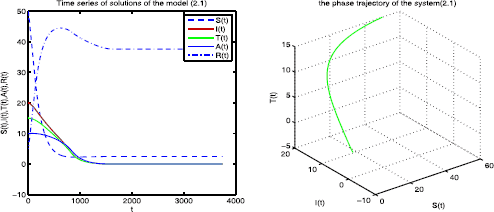

  

  The disease-free equilibrium $\pmb{E_{0}}$ is globally asymptotically stable.

• (2) When $\alpha=0.1$, $\mu_{1}=0.03$, $k_{1}=0.15$, $k_{2}=0.35$. By directly computing, we have $\Re_{0}=1.7787>1$, $E^{*}=(7.328, 2.363, 1.592, 3.352, 11.22)$ and $\mu_{1}=0.03< k_{1}+k_{2}=0.5$. So the conditions of Theorem 4.4 are satisfied, then the endemic equilibrium $E^{*}$ is globally asymptotically stable (see Figure 2). This shows the disease is persistent.

  Figure 2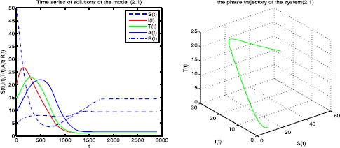

  

  The endemic equilibrium $\pmb{E_{c}}$ of the system ( 2.1 ) is globally asymptotically stable.

6 Conclusion

In this paper, a simple model HIV/AIDS epidemic model in which we consider a nonlinear incidence rate with a general form is introduced. The global dynamics of our model is determined by the basic reproduction number $\Re_{0}$. When $\Re_{0}$ is less than unity, the disease-free equilibrium is globally asymptotically stable. When $\Re_{0}$ is bigger than 1, the unique endemic equilibrium is globally asymptotically stable under the condition $\mu _{1}< k_{1}+k_{2}$. Our results suggest that appreciable change in the susceptible individuals’ sexual habits faster reduces both incidence and prevalence the disease. Numerical simulations are given to support our analytic results.

References

Naresh, R, Tripathi, A, Omar, S: Modelling the spread of AIDS epidemic with vertical transmission. Appl. Math. Comput. 178, 262-272 (2006)
Chibaya, S, Kgosimore, M: Mathematical analysis of drug resistance in vertical transmission of HIV/AIDS. Open J. Epidemiol. 3(3), 139-148 (2013)
de Arazoza, H, Lounes, R: A non-linear model for a sexually transmitted disease with contact tracing. IMA J. Math. Appl. Med. Biol. 19, 221-234 (2002)
Naresh, R, Sharma, D: An HIV/AIDS model with vertical transmission and time delay. World J. Model. Simul. 7(3), 230-240 (2011)
Yusuf, T, Benyah, F: Optimal strategy for controlling the spread of HIV/AIDS disease: a case study of South Africa. J. Biol. Dyn. 6(2), 475-494 (2012)
Huo, HF, Chen, R, Wang, XY: Modelling and stability of HIV/AIDS epidemic model with treatment. Appl. Math. Model. 40, 6550-6559 (2016)
Ma, Z, Li, J: Dynamical Modeling and Analysis of Epidemics. World Scientific, Hackensack (2009)
Li, XB, Yang, LJ: Stability analysis of an SEIQV epidemic model with saturated incidence rate. Nonlinear Anal., Real World Appl. 13, 2671-2679 (2012)
Liu, WM, Levin, SA, Iwasa, Y: Influence of nonlinear incidence rates upon the behavior of SIRS epidemiological models. J. Math. Biol. 23, 187-204 (1986)
Hethcote, HW, van den Driessche, P: Some epidemiological models with nonlinear incidence. J. Math. Biol. 29, 271-287 (1991)
Li, JQ, Yang, YL, Wu, JH, Song, XC: Global stability of vaccine-age/staged-structured epidemic models with nonlinear incidence. Electron. J. Qual. Theory Differ. Equ. 2016, 18 (2016)
Korobeinikov, A: Global properties of infection disease models with nonlinear incidnce. Bull. Math. Biol. 69, 1871-1896 (2007)
Korobeinikov, A, Maini, PK: Non-linear incidence and stability of infections disease models. Math. Med. Biol. 22, 113-128 (2005)
Muldowney, JS: Dichotomies and asymptotic behaviour for linear differential systems. Trans. Am. Math. Soc. 283, 465-584 (1984)
Li, MY, Muldowney, JS: Global stability for the SEIR model in epidemiology. Math. Biosci. 125, 155-164 (1995)
Li, MY, Wang, LC: Global stability in some SEIR epidemic models. In: Mathematical Approaches for Emerging and Reemerging Infectious Diseases: Models, Methods, and Theory. The IMA Volumes in Mathematics and Its Applications, vol. 126, pp. 295-311. Springer, New York (2002)
van den Driessche, P: Reproduction numbers and sub-threshold endemic equilibria for compartmental models of disease transmission. Math. Biosci. 180, 29-48 (2002)
Gautam, R: Reproduction numbers for infections with free-living pathogens growing in the environment. J. Biol. Dyn. 6(2), 923-940 (2012)
Perko, L: Differential Equations and Dynamical Systems, 3rd edn. Springer, New York (2001)
Kelley, WG, Peterson, AC: The Theory of Differential Equations: Classical and Qualitative, 2nd edn. Springer, New York (2010)
Sun, CJ, Lin, YP, Tang, SP: Global stability for an special SEIR epidemic model with nonlinear incidence rates. Chaos Solitons Fractals 33(1), 290-297 (2007)
Freedman, HI, Ruan, SG, Tang, M: Uniform persistence and ows near a closed positively invariant set. J. Dyn. Differ. Equ. 6, 583-600 (1994)
Smith, HL: Systems of ordinary differential equations which generate an order preserving flow. SIAM Rev. 30, 87-113 (1988)
Acknowledgements
We greatly appreciate the editor and the anonymous referees careful reading and valuable comments, their critical comments and helpful suggestions greatly improve the presentation of this paper. This work is supported by Natural Science Foundation of Shanxi province (2013011002-2).
Author information
Authors and Affiliations
Corresponding author
Additional information
Competing interests
The authors declare that they have no competing interests.
Authors’ contributions
All authors contributed equally to the writing of this paper. The authors read and approved the final manuscript.
Publisher’s Note
Springer Nature remains neutral with regard to jurisdictional claims in published maps and institutional affiliations.
Rights and permissions
Open Access This article is distributed under the terms of the Creative Commons Attribution 4.0 International License (http://creativecommons.org/licenses/by/4.0/), which permits unrestricted use, distribution, and reproduction in any medium, provided you give appropriate credit to the original author(s) and the source, provide a link to the Creative Commons license, and indicate if changes were made.
About this article
Cite this article
Jia, J., Qin, G. Stability analysis of HIV/AIDS epidemic model with nonlinear incidence and treatment. Adv Differ Equ 2017, 136 (2017). https://doi.org/10.1186/s13662-017-1175-5
Received:
Accepted:
Published:
DOI: https://doi.org/10.1186/s13662-017-1175-5