Bifurcation for model of the ³He-⁴He liquid mixture

Abstract

Experiments show that the liquid mixture of helium-3 and helium-4 has either a superfluid phase or phase separation when the temperature decreases or the mole fraction of helium-3 changes. In this paper, we investigate the equations which govern these phase transitions and derive the criteria for these phase changes; we also give an approximate solution of each phase.

1 Introduction

Liquid helium-3 and helium-4 can be dissolved into each other. Experiments show that this mixture has either a superfluid phase or phase separation when the temperature decreases or the mole fraction of helium-3 changes. In one of these experiments, the liquid mixture of ³He and ⁴He is put into a certain container, and the temperature T is lowered. Then the critical temperature of superfluidity or phase separation is recorded. After a series of experiments, the critical temperature is found to be relevant to the blending ratio of the liquid helium mixture. Assume that total mole density of the mixture is 1, and let X ($0\leq X\leq1$) be the mole fraction of helium-3 (i.e. $1-X$ is the mole fraction of helium-4), then the blending ratio of the mixture can be determined by X. Thus we have a phase diagram as below; see Figure 1 [1].

Figure 1

Experiment result.

In this diagram (Figure 1), the parameter set $\{ (X,T)|T>0, 0< X<1\}$ is divided into three disjoint regions. When the control parameter $(X,T)$ is in a certain region, the corresponding phase described in the diagram can be observed in the experiment. In this paper, we intend to give this conclusion from the mathematical point of view.

The behaviour of the ³He-⁴He liquid mixture is governed by the following equations (see [1]):

$$ \textstyle\begin{cases} \frac{\partial\psi}{\partial t}=\mu_{1}\triangle\psi-\lambda_{1}\psi -\gamma_{2}|\psi|^{2}\psi-2\nu_{4}u\psi &\mbox{in }\Omega, \\ \frac{\partial u}{\partial t}=-\mu_{2}\triangle^{2} u+\lambda _{2}\triangle u+\triangle[(-\nu_{2}+\nu_{3} X) u^{2}+\nu_{3} u^{3}+\nu _{4}|\psi|^{2}] &\mbox{in }\Omega, \\ \int_{\Omega}u \,dx=0. \end{cases} $$

(1)

In these equations, $\psi=\psi^{1}+i\psi^{2}$ describes the superfluidity of helium-4; u is the mole density of helium-3; $\mu _{1},\mu_{2},\gamma_{2},\nu_{2},\nu_{3},\nu_{4}>0$ are parameters irrelevant to $(X,T)$. We have

$$ \begin{aligned} &\lambda_{1}=-\sigma_{1}+ \theta_{2} T+\sigma_{1} X, \\ &\lambda_{2}=\theta_{1}(T+\sigma_{0})- \frac{2a\theta_{1}}{R}(1-X)X, \end{aligned} $$

(2)

where R is the molar gas constant; $a,\theta_{1},\theta_{2}>0$ are constants; $\sigma_{0},\sigma_{1}>0$ are small correction terms.

Ω describes the occupied area of the container. For simplicity, we assume $L>l$, and let $\Omega=(0,L)\times(0,l)\times(0,l)\subset \mathbb{R}^{3}$. So L, the longest edge of the container, determines its size.

The boundary condition is given by

$$\frac{\partial u}{\partial n}=0,\qquad \frac{\partial\triangle u}{\partial n}=0,\qquad \frac{\partial\psi}{\partial n}=0\quad \mbox{on }\partial\Omega. $$

Equations (1) admit a solution $\psi=0$, $u=0$, which refers to the normal phase. Meanwhile, $\psi\neq0$, $u=0$ refers to superfluidity of helium-4; $\psi=0$, $u\neq0$ refers to phase separation; and $\psi \neq0$, $u\neq0$ refers to superfluidity and phase separation. So we are focussed on nonzero solutions for (1).

Two critical curves in the XT-plane were given by Ma and Wang in [1]. They also derived corresponding phase diagrams and an expression of one bifurcation.

In this paper, we discuss the steady state equations of (1) with $(X,L,T)$ as the control parameter, where X is the mole fraction of helium-3, L is the longest edge of the container, and T is the temperature. And here is our task:

• 1. give a different critical curve;

• 2. provide phase diagrams in the LT-plane and a different phase diagram in the XT-plane;

• 3. derive the expression of other bifurcating solutions.

See [2–13] for more studies on bifurcation problems or the behaviour of liquid helium.

The remainder of this paper is organised as follows. In Section 2 we give preliminaries. In Section 3 we give the critical curves and phase diagram. In Section 4 we give solutions corresponding to each phases. In Section 5 we give the proofs.

2 Preliminaries

In this section, we give a brief review of Ma and Wang’s dynamic transition theory. We rewrite (1) as a two operator equation.

2.1 Dynamic transition theory

Consider the following operator equation:

$$ \frac{dw}{dt}=\mathcal{L}_{\Lambda} w+\mathcal{G}(w). $$

(3)

Here w is the unknown; $\mathcal{L}_{\Lambda}$ is a family of linear operators, with $\{\beta_{i}(\Lambda)\}$ as eigenvalues (listed by algebraic multiplicities); Λ is the control parameter; and $\mathcal{G}(w)=o(|w|)$. Assume that there is $\Lambda_{0}$ such that $\{ \beta_{i}(\Lambda)\}$ satisfies the following. For $j\geqslant m+1$, $\operatorname{Re}\beta_{j}(\Lambda_{0})<0$, and for $1\leqslant i\leqslant m$,

$$\begin{aligned}& \operatorname{Re}\beta_{i}(\Lambda)< 0 \quad\mbox{if }\Lambda< \Lambda_{0}, \\& \operatorname{Re}\beta_{i}(\Lambda)=0\quad \mbox{if }\Lambda= \Lambda_{0}, \\& \operatorname{Re}\beta_{i}(\Lambda)>0\quad \mbox{if }\Lambda> \Lambda_{0}. \end{aligned}$$

Then equation (3) will undergo a transition at $\Lambda =\Lambda_{0}$. In other words, the solution $w=0$ is stable when $\Lambda< \Lambda_{0}$; and when $\Lambda> \Lambda _{0}$, it is not stable.

To illustrate, let $\Lambda=(X,T)$ and $\beta(X,T)$ be first eigenvalue of $\mathcal{L}_{\Lambda}$. Then $\{(X,T)|\beta=0\}$ defines a curve in the XT-plane. This curve is called critical curve, it divides the XT-plane into two disjoint regions $\{(X,T)|\beta<0\}$ and $\{ (X,T)|\beta>0\}$. And each region refers to a different phase state. In other words, as the control parameters $(X,T)$ cross the critical curve $\{(X,T)|\beta=0\}$ (i.e. from $\{(X,T)|\beta<0\}$ to $\{ (X,T)|\beta>0\}$), a transition takes place.

2.2 Operator equations

Following this idea, let $\Lambda =(X,L,T)$, and we will rewrite equation (1) as two operator equations. Note that $\lambda_{1,2}=\lambda_{1,2}(X,T)$; see (2).

Denote $w=(\psi^{1},\psi^{2},u)^{T}$, and

$$\mathrm{H}=\biggl\{ w\in\mathrm{H}^{4}\bigl(\Omega, \mathbb{R}^{3}\bigr)\Big| \int_{\Omega}u=0, \frac{\partial u}{\partial n}\bigg|_{\partial\Omega}=0, \frac{\partial \triangle u}{\partial n}\bigg|_{\partial\Omega}=0, \frac{\partial\psi ^{1,2}}{\partial n}\bigg|_{\partial\Omega}=0\biggr\} . $$

Consider the operators $\mathcal{L}^{1}_{\Lambda}:\mathrm{H}\rightarrow \mathrm{L}^{2}(\Omega,\mathbb{R}^{3})$ and $\mathcal{G}:\mathrm{H}\rightarrow\mathrm{L}^{2}(\Omega,\mathbb {R}^{3})$, where

$$\begin{aligned}& \mathcal{L}^{1}_{\Lambda}=\left ( \textstyle\begin{array}{@{}c@{\quad}c@{\quad}c@{}} \mu_{1}\triangle-\lambda_{1} & 0 & 0 \\ 0 & \mu_{1}\triangle-\lambda_{1} & 0 \\ 0 & 0 & -\mu_{2}\triangle^{2}+\lambda_{2}\triangle \end{array}\displaystyle \right ) , \\& \mathcal{G}(w)=\left ( \textstyle\begin{array}{@{}c@{}} \mathcal{G}_{1}(w)\\ \mathcal{G}_{2}(w)\\ \mathcal{G}_{3}(w) \end{array}\displaystyle \right ) =\left ( \textstyle\begin{array}{@{}c@{}} -\gamma_{2}|\psi|^{2}\psi^{1}-2\nu_{4}u\psi^{1}\\ -\gamma_{2}|\psi|^{2}\psi^{2}-2\nu_{4}u\psi^{2}\\ \triangle[(-\nu_{2}+\nu_{3} X) u^{2}+\nu_{3} u^{3}+\nu_{4}|\psi |^{2}] \end{array}\displaystyle \right ) . \end{aligned}$$

Then the steady state equations of (1) can be rewritten as

$$ \mathcal{L}^{1}_{\Lambda}w+\mathcal{G}(w)=0. $$

(4)

If $\lambda_{1}<0$, then steady state equations of (1) admit a solution (see [1]),

$$\psi= \sqrt{-\lambda_{1} / \gamma_{2}}e^{i \phi}, \qquad u=0,\quad \phi\in[0, 2\pi). $$

Equation (1) is invariant when we apply an orthogonal transformation, so $\phi=0$ in a properly chosen coordinate system of $\mathbb{C}$. Note that we always assume this coordinate system in this paper.

Consequently, this solution can be rewritten as

$$ \psi= \sqrt{-\lambda_{1} / \gamma_{2}},\qquad u=0 . $$

(5)

Denote $\widetilde{w}=(\psi^{1}-\sqrt{-\lambda_{1} / \gamma_{2}},\psi ^{2},u)^{T}$, we rewrite equations (1) as

$$ \mathcal{L}^{2}_{\Lambda}\widetilde{w}+\mathcal{J}( \widetilde{w})=0. $$

(6)

Here operators $\mathcal{L}^{2}_{\Lambda}:\mathrm{H}\rightarrow\mathrm {L}^{2}(\Omega,\mathbb{R}^{3})$ and $\mathcal{J}:\mathrm{H}\rightarrow\mathrm{L}^{2}(\Omega,\mathbb {R}^{3})$ can be expressed as follows:

$$\mathcal{L}^{2}_{\Lambda}=\left ( \textstyle\begin{array}{@{}c@{\quad}c@{\quad}c@{}} \mu_{1}\triangle+2\lambda_{1} & 0 & -\nu_{4}\sqrt{-\lambda_{1} /\gamma_{2}} \\ 0 & \mu_{1}\triangle& 0 \\ -2\nu_{4}\sqrt{-\lambda_{1} /\gamma_{2}} & 0 & -\mu_{2}\triangle^{2}+\lambda _{2}\triangle \end{array}\displaystyle \right ) ,\qquad\mathcal{J}=(\mathcal{J}_{1}, \mathcal{J}_{2}, \mathcal{J}_{3})^{T}, $$

where

$$\begin{aligned}& \mathcal{J}_{1}(\widetilde{w}) = -3\gamma_{2}\sqrt{- \lambda_{1}/\gamma_{2}}\psi _{1}^{2}- \gamma_{2}\sqrt{-\lambda_{1}/\gamma_{2}} \psi_{2}^{2}- 2\nu_{4}u\psi_{1}- \gamma _{2}\psi_{1}^{3}-\gamma_{2} \psi_{2}^{2}\psi_{1}, \\& \mathcal{J}_{2}(\widetilde{w}) = -2\gamma_{2}\sqrt{- \lambda_{1}/\gamma_{2}}\psi _{1}\psi_{2}- 2\nu_{4}u\psi_{2}- \gamma_{2}\psi_{2}^{3}- \gamma_{2}\psi_{1}^{2}\psi_{2}, \\& \mathcal{J}_{3}(\widetilde{w}) = \triangle\bigl[(-\nu_{2}+ \nu_{3} X) u^{2}+\nu _{3} u^{3}+ \nu_{4}\psi_{1}^{2}+\nu_{4} \psi_{2}^{2}\bigr]. \end{aligned}$$

3 Critical curves and phase diagram

In this section we will introduce three critical curves; and give theoretical phase diagrams.

Let $\beta_{1}$ and $\beta_{2}$ be the first two eigenvalues of $\mathcal {L}^{1}_{\Lambda}$, then

$$\begin{aligned}& \beta_{1} =-\lambda_{1}=\sigma_{1}- \theta_{2} T- \sigma_{1} X , \\& \beta_{2} =-\frac{\pi^{2}}{L^{2}}\biggl[\frac{\pi^{2}}{L^{2}} \mu_{2}+\theta _{1}T+\theta_{1}\sigma_{0}+ \frac{2a\theta_{1}}{R}X(X-1)\biggr]. \end{aligned}$$

Let $\beta_{3}$ be the first eigenvalue of $\mathcal{L}^{2}_{\Lambda}$, and we have

$$ \beta_{3}=\frac{1}{2}\bigl(D+ \sqrt{D^{2}-4B}\bigr), $$

(7)

where

$$\begin{aligned}& D =-\frac{\pi^{2}}{L^{2}}\mu_{1}+2\lambda_{1}-\mu_{2} \frac{\pi^{4}}{L^{4}}-\frac{\pi ^{2}}{L^{2}}\lambda_{2}, \\& B =-\frac{\pi^{2}}{L^{2}}\biggl(-\frac{\pi^{2}}{L^{2}}\mu_{1}+2 \lambda_{1}\biggr) \biggl(\frac{\pi ^{2}}{L^{2}}\mu_{2}+ \lambda_{2}\biggr)-\frac{\pi^{2}}{L^{2}}\bigl(4\nu_{4}^{2}/ \gamma_{2}\bigr)\lambda_{1}. \end{aligned}$$

Following the idea mentioned in Section 2, we derive three functions as follows:

$$\begin{aligned} &\beta_{1}=0 \quad\Leftrightarrow\quad T=T_{C1}, \\ &\beta_{2}=0\quad\Leftrightarrow\quad T=T_{C2}, \\ &\beta_{3}=0\quad\Leftrightarrow\quad T=T_{C3}. \end{aligned} $$

The formulae of $T=T_{C1}$ and $T=T_{C2}$ were given by (see [1])

$$ \begin{aligned} &T=T_{C 1} = \frac{\sigma_{1}}{\theta_{2}}(1-X), \\ &T=T_{C 2} = \frac{2a}{R}X(1-X)-\frac{\mu_{2} \pi^{2}}{\theta_{1} L^{2}}- \sigma_{0}. \end{aligned} $$

(8)

$T=T_{C3}$ can be expressed by the following lemma.

Lemma 3.1

The formula of $T=T_{C3}$ can be written as

$$\begin{aligned} T={}&T_{C3} \\ ={}&\frac{1}{2}(1-X) \biggl( \frac{2a}{R}X+ \frac{\sigma_{1}}{\theta_{2}}\biggr)+ \frac{\pi^{2}}{4\theta_{1} L^{2}}( \mu_{1}-2\mu_{2} )- \frac{\sigma_{0}}{2}+ \frac {\nu_{4}^{2}}{\theta_{1} \gamma_{2}} \\ &{}- \frac{1}{4\theta_{1}\theta_{2}} \biggl\{ \biggl[ 2\theta_{1}\theta _{2}(1-X) \biggl(\frac{2a}{R}X- \frac{\sigma_{1}}{\theta_{2}}\biggr)- 2 \theta_{1}\theta _{2}\sigma_{0}- \frac{4\theta_{2}\nu_{4}^{2}}{\gamma_{2}}- \frac{\pi^{2}}{L^{2}}(2\theta _{2}\mu_{2}+ \theta_{1}\mu_{1}) \biggr]^{2} \\ &{}+ \frac{32\theta_{1}\theta_{2}^{2}\nu_{4}^{2}}{\gamma_{2}} \biggl[(1-X) \biggl(\frac {2a}{R}X- \frac{\sigma_{1}}{\theta_{2}}\biggr)-\frac{\mu_{2}\pi^{2}}{\theta_{1} L^{2}}-\sigma_{0} \biggr] \biggr\} ^{1/2}. \end{aligned}$$

(9)

Moreover, if $T_{C2}< T_{C1}$, then $T_{C2}< T_{C3}< T_{C1}$; if $T=T_{C 1}$ and $T=T_{C 2}$ intersect in a point $(X_{0},L_{0},T_{0})$, then $T_{0}=T_{C 3}(X_{0},L_{0})$. See Figures  2, 3 and  5.

Figure 2

4-phase.

Figure 3

3-phase.

Proof

If $T_{C2}< T_{C1}$, then $D<0$. Consequently, $\beta _{3} =0$ if and only if $B=0$. And we can rewrite $B=0$ as either of the following:

$$ \begin{aligned} &2\theta_{1}\theta_{2}(T -T_{C2})^{2}+ \bigl[2\theta_{1}\theta _{2}(T_{C2}-T_{C1})-2\theta_{2}\bigl(2 \nu_{4}^{2}/\gamma_{2}\bigr)-\bigl(\mu_{1}\pi^{2}/L^{2}\bigr) \theta_{1}\bigr](T-T_{C2}) \\ &\quad{} - 2\theta_{2}\bigl(2 \nu_{4}^{2}/\gamma _{2}\bigr) (T_{C2}-T_{C1})=0, \\ &2\theta_{1}\theta_{2}(T -T_{C1})^{2}+ \bigl[2\theta_{1}\theta _{2}(T_{C1}-T_{C2})-2 \theta_{2}\bigl(2\nu_{4}^{2}/\gamma_{2} \bigr)-\bigl(\mu_{1}\pi^{2}/L^{2}\bigr) \theta_{1}\bigr](T-T_{C1}) \\ &\quad{} - \theta_{1}\bigl( \mu_{1}\pi ^{2}/L^{2}\bigr) (T_{C1}-T_{C2})=0. \end{aligned} $$

(10)

Assume $T_{C2}< T_{C1}$. According to the Viète theorem and (10), we derive Lemma 3.1 naturally. □

The following lemma gives more information as regards the eigenvalues and the critical curves.

Lemma 3.2

$$\beta_{i}< 0 \quad\Leftrightarrow\quad T>T_{Ci},\qquad \beta_{i}>0 \quad\Leftrightarrow\quad T< T_{Ci},\quad i=1,2. $$

Meanwhile, if $T_{C2}< T< T_{C1}$, then

$$\beta_{3}< 0 \quad\Leftrightarrow\quad T>T_{C3},\qquad \beta_{3}>0 \quad\Leftrightarrow\quad T< T_{C3}. $$

Proof

The first conclusion is trivial. We have $D=-\frac{\pi^{2}}{L^{2}}\mu _{1}-2\beta_{1}+\beta_{2}$. If $T_{C2}< T< T_{C1}$, then $\beta_{1}>0$, $\beta_{2}<0$, which means $D<0$. Then we derive the second conclusion naturally. □

We have to decide which one of $\beta_{1}$ and $\beta_{2}$ is the first eigenvalue of $\mathcal{L}^{1}_{\Lambda}$. In other words, we should distinguish whether $T_{C1}< T_{C2}$ or $T_{C1}>T_{C2}$. Meanwhile the greatest value of $T_{C3}$ may be less than zero or not. According to these possibilities, we have several different phase diagrams.

First we consider $(L,T)$ as the control parameter, where L is the longest edge of the container and T is the temperature, as in Section 1. Then we derive three different phase diagrams in the LT-plane.

• 1. If $T=T_{C1}$ and $T=T_{C2}$ intersect, then we have the 4-phase diagram; see Figure 2.

• 2. If $T=T_{C1}$ and $T=T_{C2}$ do not intersect and $\max T_{C3}>0$, then we have a 3-phase diagram; see Figure 3.

• 3. If $\max T_{C3}\leqslant0$, then we have a 2-phase diagram; see Figure 4.

  Figure 4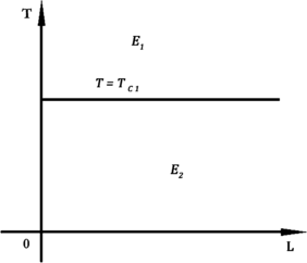

  

  2-phase.

Likewise, consider phase diagrams in the XT-plane, where X is the mole fraction of helium-3. We only introduce the phase diagram in the case that the critical curves $T=T_{C1}$ and $T=T_{C2}$ intersect in two points. See Figure 5. The other cases are similar. Note that this diagram agrees with the physical phase diagram; see Figure 1.

Figure 5

Two intersections.

In all these four phase diagrams, $E_{1}$ is the normal phase region; $E_{2}$ is the superfluid phase region; $E_{3}$ is the phase separation region; and in region $E_{4}$ superfluidity and phase separation both take place. The formulae of solutions in each regions will be given in the next section. It is worth to mention that there is a different critical curve $T=T_{C4}$, but we failed to give its formula.

4 Bifurcating solutions of phase transition

4.1 Eigenvalues and eigenvectors

The first phase transition is governed by the operator equation (4), and the second phase transition is governed by the operator equation (6). For our further argument, we need all the eigenvalues and eigenvectors of $\mathcal{L}^{1}_{\Lambda}$ and $\mathcal{L}^{2}_{\Lambda}$.

Assume

$$\begin{aligned}& \eta_{\alpha}=-\biggl(\frac{\alpha_{1} \pi}{L}\biggr)^{2}-\biggl( \frac{\alpha_{2} \pi }{l}\biggr)^{2}-\biggl(\frac{\alpha_{3} \pi}{l} \biggr)^{2}, \\& \varphi_{\alpha}=\cos\frac{\alpha_{1}\pi x_{1}}{L}\cos\frac{\alpha_{2}\pi x_{2}}{l}\cos \frac{\alpha_{3}\pi x_{3}}{l}. \end{aligned}$$

Here $\alpha=(\alpha_{1},\alpha_{2},\alpha_{3})$ is a multi-index and $|\alpha |=\alpha_{1}+\alpha_{2}+\alpha_{3}$.

Then the eigenvalues of $\mathcal{L}^{1}_{\Lambda}$ are given by

$$ \beta^{1,2}_{\alpha}=\mu_{1} \eta_{\alpha}-\lambda_{1},\quad |\alpha |=0,1,2,\ldots,\qquad \beta^{3}_{\alpha}=-\mu_{2}(\eta_{\alpha})^{2}+ \lambda_{2}\eta_{\alpha},\quad |\alpha |=1,2,\ldots. $$

(11)

The eigenvectors of $\mathcal{L}^{1}_{\Lambda}$ corresponding to $\beta ^{1,2,3}_{\alpha}$ can be expressed as

$$\begin{aligned} &\Phi^{1}_{\alpha}=(\varphi_{\alpha},0,0)^{T}, \quad |\alpha|=0,1,2,\ldots, \\ &\Phi^{2}_{\alpha}=(0,\varphi_{\alpha},0)^{T}, \quad |\alpha|=0,1,2,\ldots, \\ &\Phi^{3}_{\alpha}=(0,0,\varphi_{\alpha})^{T}, \quad |\alpha|=1,2,\ldots. \end{aligned} $$

Meanwhile, the eigenvalues of $\mathcal{L}^{2}_{\Lambda}$ are given by

$$ \begin{aligned} &\xi_{0} = 2\lambda_{1}, \\ &\xi_{\alpha}^{1} = \mu_{1}\eta_{\alpha},\quad | \alpha|\geqslant1, \\ &\xi_{\alpha}^{2} = \frac{1}{2}\Bigl(D_{\alpha}+ \sqrt{D_{\alpha}^{2}-4B_{\alpha }}\Bigr),\quad | \alpha|\geqslant1, \\ &\xi_{\alpha}^{3} = \frac{1}{2}\Bigl(D_{\alpha}- \sqrt{D_{\alpha}^{2}-4B_{\alpha }}\Bigr),\quad | \alpha|\geqslant1, \end{aligned} $$

(12)

where

$$\begin{aligned}& D_{\alpha} = \mu_{1}\eta_{\alpha}+2\lambda_{1}- \mu_{2}\eta_{\alpha}^{2}+\lambda _{2} \eta_{\alpha}, \\ & B_{\alpha} = (\mu_{1}\eta_{\alpha}+2\lambda_{1}) \bigl(-\mu_{2}\eta_{\alpha }^{2}+\lambda_{2} \eta_{\alpha}\bigr)-\bigl(4\nu_{4}^{2}/ \gamma_{2}\bigr)\lambda_{1}\eta_{\alpha}. \end{aligned}$$

Note that we only consider eigenvalues that are real numbers here, for no bifurcation will happen if they are imaginary numbers.

The eigenvectors of $\mathcal{L}^{2}_{\Lambda}$ and eigenvectors of its conjugation operator $\mathcal{L}^{2}_{\Lambda}$ can be expressed as

$$\begin{aligned}& \Gamma_{0}=(1,0,0)^{T}, \qquad(\Gamma_{0})^{*}=\biggl(1,0, \frac{\nu_{4}}{2}\sqrt{\frac {1}{\beta_{1}\gamma_{2}}}\biggr)^{T}, \\ & \Gamma_{\alpha}^{1}=(0,\varphi_{\alpha},0)^{T}, \qquad \bigl(\Gamma_{\alpha }^{1}\bigr)^{*}=(0,\varphi_{\alpha},0)^{T},\quad |\alpha|\geqslant1, \\ & \Gamma_{\alpha}^{2}=\bigl(\varphi_{\alpha},0,y_{\alpha}^{2} \varphi_{\alpha }\bigr)^{T}, \qquad\bigl(\Gamma_{\alpha}^{2}\bigr)^{*}=\bigl(\varphi_{\alpha},0,\bigl(y_{\alpha}^{2}\bigr)^{*} \varphi_{\alpha}\bigr)^{T},\quad |\alpha|\geqslant1, \\ & \Gamma_{\alpha}^{3}=\bigl(\varphi_{\alpha},0,y_{\alpha}^{3} \varphi_{\alpha }\bigr)^{T}, \qquad\bigl(\Gamma_{\alpha}^{3}\bigr)^{*}=\bigl(\varphi_{\alpha},0,\bigl(y_{\alpha}^{3}\bigr)^{*} \varphi_{\alpha}\bigr)^{T},\quad |\alpha|\geqslant1. \end{aligned}$$

Here

$$\begin{aligned}& y_{\alpha}^{2,3} =\frac{\mu_{1} \eta_{\alpha}+2\lambda_{1}-\xi_{\alpha }^{2,3}}{2\nu_{4}\sqrt{-\lambda_{1}/\gamma_{2}}}, \\ & \bigl(y_{\alpha}^{2,3}\bigr)^{*} =-\frac{\mu_{1} \eta_{\alpha}+2\lambda_{1}-\xi_{\alpha }^{2,3}}{2\nu_{4}\eta_{\alpha}\sqrt{-\lambda_{1}/\gamma_{2}}}. \end{aligned}$$

4.2 Solutions

First we introduce the following parameters:

$$ \begin{aligned} &A=\frac{\pi^{4}}{L^{3} \beta^{3}_{(2,0,0)}}(-\nu_{2}+3 \nu_{3} X)^{2}+\frac{3\pi ^{2}}{8L}\nu_{3}, \\ &N_{0}=\frac{Ll^{2}}{4\lambda_{1}} ( 3\sqrt{-\lambda_{1} \gamma_{2}}+2\nu_{4} ), \\ &N_{i}=\frac{\frac{1}{2}(3\sqrt{-\lambda_{1}\gamma_{2}}+2\nu_{4} )+\frac{2\pi ^{2}}{L^{2}}y_{(2,0,0)}^{i}(-\nu_{2}+3\nu_{3} X+\nu_{4})}{ (1+y_{(2,0,0)}^{i}(y_{(2,0,0)}^{i})^{*})\xi_{(2,0,0)}^{i}},\quad i=2,3, \\ &M=\frac{1}{1+y_{(1,0,0)}^{2}(y_{(1,0,0)}^{2})^{*}} \biggl\{ \biggl[ 2(3\sqrt {-\lambda_{1} \gamma_{2}}+\nu_{4} )N_{0}+(3\sqrt{- \lambda_{1}\gamma_{2}}+\nu_{4} ) (N_{2}+N_{3}) \\ &\hphantom{M={}}{}+\nu_{4}\bigl(y_{(2,0,0)}^{2}N_{2}+y_{(2,0,0)}^{3}N_{3} \bigr)+\frac{3}{2}\gamma_{2} \biggr]+\frac{\pi^{2}}{L^{2}} \bigl[2 \nu_{4}N_{0}+3\nu_{4}(N_{2}+N_{3}) \\ &\hphantom{M={}}+3(-\nu_{2}+3\nu_{3} X) \bigl(y_{(2,0,0)}^{2}N_{2}+y_{(2,0,0)}^{3}N_{3} \bigr)-3 \bigr] \biggr\} . \end{aligned} $$

(13)

Then we have two theorems for equations (1), which give solutions corresponding to each phase of the ³He-⁴He mixture. Note that we always assume a properly chosen coordinate system of $\mathbb{C}$; see (5).

The first transition takes place at $T=T_{C 1}$ or $T=T_{C 2}$. The formula of the bifurcation from $T=T_{C 1}$ (i.e., the solution in region $E_{2}$; see Figures 2, 3, 4 and 5) is given by

$$\psi= \sqrt{-\lambda_{1} / \gamma_{2}},\qquad u=0. $$

The transition at $T=T_{C 2}$ is described by the following theorem (i.e., $E_{1}$ to $E_{3}$; see Figures 2 and 5).

Theorem 4.1

For each $(X_{0},L_{0}, T_{0})\in\{(X,L,T)|T=T_{C2}, T_{C1}< T_{C2}, 0\leqslant X\leqslant1, L>0, T\geqslant0\}$, there is some ε such that, for all $0<(X-X_{0})^{2}+(L-L_{0})^{2}+(T-T_{0})^{2}<\varepsilon$, the steady state equations of (1) have a bifurcation from $(\psi ,u,X,L,T)=(0,0, X_{0}, L_{0}, T_{0})$, which can be expressed as

$$ \psi=0,\qquad u=\pm \biggl(\frac{L}{2A}\beta_{2} \biggr)^{\frac{1}{2}} \cos\frac {\pi x_{1}}{L}+o \bigl(\beta_{2}^{\frac{1}{2}} \bigr). $$

(14)

Here $\beta_{2}=\beta_{(1,0,0)}^{3}$ is the eigenvalue of $\mathcal {L}^{1}_{\Lambda}$; see (11).

The second transition takes place at $T=T_{C 3}(X)$ (i.e., $E_{2}$ to $E_{4}$; see Figures 2, 3 and 5). Before that, the first transition at $T=T_{C 1}$ already happened. From the physical point of view, superfluidity is observed before phase separation.

Theorem 4.2

For each $(X_{0},L_{0}, T_{0})\in\{(X,L,T)|T=T_{C3}, T_{C2}< T_{C1}, 0\leqslant X\leqslant1, L>0, T\geqslant0\}$, there is some ε such that for all $0<(X-X_{0})^{2}+(L-L_{0})^{2}+(T-T_{0})^{2}<\varepsilon$, the steady state equations of (1) have a bifurcation from $( (-\lambda_{1} / \gamma_{2} )^{\frac{1}{2}},0, X_{0}, L_{0}, T_{0})$, which can be expressed as

$$ \begin{aligned} &\psi^{\pm} = \biggl(\frac{-\lambda_{1}}{\gamma_{2}} \biggr)^{\frac {1}{2}}\pm \biggl(\frac{\beta_{3}}{M} \biggr)^{\frac{1}{2}} \cos{ \frac{\pi x_{1}}{L}}+o \bigl(\beta_{3}^{\frac{1}{2}} \bigr), \\ &u^{\pm} = \pm y_{(1,0,0)}^{2} \biggl(\frac{\beta_{3}}{M} \biggr)^{\frac {1}{2}}\cos\frac{\pi x_{1}}{L}+o \bigl(\beta_{3}^{\frac{1}{2}} \bigr). \end{aligned} $$

(15)

Here $\beta_{3}=\xi_{(1,0,0)}^{2}$ is the first eigenvalue of $\mathcal {L}^{2}_{\Lambda}$; see (7).

Thus, we have a solution corresponding to each phase as follows:

• 1. In the normal phase region $E_{1}$, we have $(\psi,u)=( 0,0)$.

• 2. In the superfluid phase region $E_{2}$, we have $(\psi,u)=( \sqrt {-\lambda_{1} / \gamma_{2}},0)$.

• 3. When $A>0$, we have $(\psi, u)= (0, \pm (\frac{L}{2A}\beta _{2} )^{\frac{1}{2}} \cos\frac{\pi x_{1}}{L}+o (\beta_{2}^{\frac {1}{2}} ) )$ in region $E_{3}$, which means that phase separation takes place.

• 4. When $M>0$, we have $(\psi,u)=(\psi^{\pm},u^{\pm})$ in region $E_{4}$, which means superfluidity and phase separation both can be observed.

5 Proofs

By the Lyapunov-Schmidt procedure [1, 6], we will prove bifurcation theorems in this section.

Proof of Theorem 4.1

By the spectral theorem of completely continuous fields [6, 14], $\{\Phi_{\alpha}^{1,2,3}\}$ is a basis set of space H and any $w \in\mathrm{H}$ can be written as

$$w=\sum_{|\alpha|=0}^{\infty}\bigl( \psi^{1}_{\alpha}\Phi^{1}_{\alpha}\bigr)+\sum _{|\alpha|=0}^{\infty}\bigl(\psi^{2}_{\alpha} \Phi^{2}_{\alpha}\bigr) +\sum_{|\alpha|=1}^{\infty} \bigl(u_{\alpha}\Phi^{3}_{\alpha}\bigr). $$

Equivalently,

$$ \psi^{1}=\sum_{|\alpha|=0}^{\infty} \bigl(\psi^{1}_{\alpha}\varphi_{\alpha}\bigr),\qquad \psi^{2}=\sum_{|\alpha|=0}^{\infty}\bigl( \psi^{2}_{\alpha}\varphi_{\alpha}\bigr),\qquad u=\sum _{|\alpha|=1}^{\infty}(u_{\alpha} \varphi_{\alpha}). $$

(16)

It follows from (4) and (16) that

$$ \begin{aligned} &\sum_{|\alpha|=0}^{\infty} \beta_{\alpha}^{1}\psi_{\alpha}^{1}\varphi _{\alpha}+\mathbf{G}^{1}(w)=0,\quad |\alpha|=0,1,2,\ldots, \\ &\sum_{|\alpha|=0}^{\infty}\beta_{\alpha}^{2} \psi_{\alpha}^{2}\varphi _{\alpha}+\mathbf{G}^{2}(w)=0, \quad |\alpha|=0,1,2,\ldots, \\ &\sum_{|\alpha|=1}^{\infty}\beta_{\alpha}^{3} u_{\alpha}^{1}\varphi_{\alpha }+\mathbf{G}^{3}(w)=0, \quad |\alpha|=1,2,\ldots. \end{aligned} $$

(17)

Consequently, we have

$$\begin{aligned} &\frac{1}{2}Ll^{2}\beta_{2} u_{(1,0,0)}+\bigl\langle \mathcal{G}_{3}(w),\varphi _{(1,0,0)} \bigr\rangle =0, \end{aligned}$$

(18)

$$\begin{aligned} &\begin{aligned} &\langle\varphi_{\alpha}, \varphi_{\alpha}\rangle \beta_{\alpha}^{1}\psi _{\alpha}^{1}+\bigl\langle \mathcal{G}_{1}(w), \varphi_{\alpha}\bigr\rangle =0,\quad |\alpha |=0,1,2,\ldots, \\ &\langle\varphi_{\alpha},\varphi_{\alpha}\rangle \beta_{\alpha}^{2}\psi _{\alpha}^{2}+\bigl\langle \mathcal{G}_{2}(w),\varphi_{\alpha}\bigr\rangle =0,\quad |\alpha |=0,1,2,\ldots, \end{aligned} \end{aligned}$$

(19)

$$\begin{aligned} & \langle\varphi_{\alpha},\varphi_{\alpha}\rangle \beta_{\alpha}^{3} u_{\alpha}+\bigl\langle \mathcal{G}_{3}(w),\varphi_{\alpha}\bigr\rangle =0,\quad |\alpha | \geqslant0 \mbox{ and } \alpha\neq(1,0,0). \end{aligned}$$

(20)

Here, $\langle p, q \rangle\stackrel{\mathrm{def}}{=}\int_{\Omega} pq \,dx$.

We know that

$$\begin{aligned}& \beta_{1}>\beta_{\alpha}^{1,2},\quad |\alpha|=1,2, \ldots, \\& \beta_{2}>\beta_{\alpha}^{3},\quad |\alpha|\geqslant0 \mbox{ and } \alpha\neq(1,0,0). \end{aligned}$$

Hence, the bifurcation is determined by $\beta_{1}$, $\beta_{2}$. However, the bifurcation at $T=T_{C1}$ (i.e., $\beta_{1}=0$) is known; see (5). We are focussed on the case that $T=T_{C2}$ (i.e., $\beta_{2}=0$).

For each $(X_{0},L_{0},T_{0})\in\{(X,L,T)|T=T_{C2}\}$, there is a neighbourhood U of $(X_{0},L_{0},T_{0})$ such that

$$\begin{aligned}& \beta_{2}\textstyle\begin{cases} < 0& \mbox{if }(X,L,T)\in\{(X,L,T)|T>T_{C2}\}\cap\mathbf{U}, \\ =0& \mbox{if }(X,L,T)\in\{(X,L,T)|T=T_{C2}\}\cap\mathbf{U}, \\ >0& \mbox{if }(X,L,T)\in\{(X,L,T)|T< T_{C2}\}\cap\mathbf{U}, \end{cases}\displaystyle \\& \beta_{\alpha}^{3}< 0,\quad (X,L,T)\in\mathbf{U}, \mbox{else}. \end{aligned}$$

Obviously, equations (19) admit a solution $\psi_{\alpha }^{1,2}=0$. In this case, the transition is determined by (18) and (20).

By the implicit function theorem and equations (20), if $(X,L,T) \in\mathbf{U}$, then we have the following functions in a neighbourhood of $(\psi^{1},\psi^{2},u)=(0,0,0)$:

$$ u_{\alpha}=o\bigl(|u_{(1,0,0)}|\bigr),\quad |\alpha|\geqslant1 \mbox{ and } \alpha\neq(1,0,0). $$

(21)

Consequently, by (21) and equations (20), we have

$$\begin{aligned}& u_{(2,0,0)} = \frac{2\pi^{2}}{L^{2} \beta_{(2,0,0)}^{3}}(-\nu_{2} +3 \nu_{3} X) (u_{(1,0,0)})^{2}+o\bigl(|u_{(1,0,0)}|^{2} \bigr), \\& u_{\alpha} = o\bigl(|u_{(1,0,0)}|^{2}\bigr), \quad\alpha \neq(0,0,0) \mbox{ nor } (1,0,0) \mbox{ nor } (2,0,0). \end{aligned}$$

Then equation (18) can be written as

$$\frac{L}{2}\beta_{2}u_{(1,0,0)}-A(u_{(1,0,0)})^{3}+o \bigl(|u_{(1,0,0)}|^{3}\bigr)=0. $$

Here the parameter A was introduced in Section 4; see (13).

Thus, we have

$$(u_{(1,0,0)})^{2}=\frac{L \beta_{2}}{2A}+o(\beta_{2}). $$

Then by (16), a nontrivial solution of equations (4) can be expressed as

$$\psi=0,\qquad u=\pm \biggl(\frac{L}{2A}\beta_{2} \biggr)^{\frac{1}{2}} \cos\frac {\pi x_{1}}{L}+o \bigl(\beta_{2}^{\frac{1}{2}} \bigr). $$

This completes the proof of Theorem 4.1. □

Proof of Theorem 4.2

Following the same process as we mentioned above, any $w \in\mathrm{H}$ can be written as

$$\widetilde{w}=\widetilde{w}_{0}\Gamma_{0}+\sum _{|\alpha|=1}^{\infty }\bigl(\widetilde{w}^{1}_{\alpha} \Gamma^{1}_{\alpha}\bigr)+ \sum_{|\alpha|=0}^{\infty} \bigl(\widetilde{w}^{2}_{\alpha}\Gamma^{2}_{\alpha } \bigr)+\sum_{|\alpha|=1}^{\infty}\bigl( \widetilde{w}_{\alpha}\Gamma^{3}_{\alpha}\bigr). $$

And we can rewrite (6) as

$$\begin{aligned} &\xi_{0}\widetilde{w}_{0}+\bigl\langle J( \widetilde{w}), (\Gamma_{0})^{*}\bigr\rangle =0, \end{aligned}$$

(22)

$$\begin{aligned} &\begin{aligned} &\bigl\langle \Gamma_{\alpha}^{i}, \bigl(\Gamma_{\alpha}^{i}\bigr)^{*} \bigr\rangle \xi_{\alpha }^{i}\widetilde{w}_{\alpha}^{i}+ \bigl\langle J(\widetilde{w}), \bigl(\Gamma_{\alpha }^{i}\bigr)^{*}\bigr\rangle =0,\quad |\alpha|\geqslant1, i=1,3, \\ &\bigl\langle \Gamma_{\alpha}^{2}, \bigl(\Gamma_{\alpha}^{2} \bigr)^{*} \bigr\rangle \xi_{\alpha }^{2}\widetilde{w}_{\alpha}^{2}+ \bigl\langle J(\widetilde{w}), \bigl(\Gamma_{\alpha }^{2}\bigr)^{*} \bigr\rangle =0,\quad |\alpha|\geqslant1 \mbox{ and } \alpha\neq(1,0,0), \end{aligned} \end{aligned}$$

(23)

$$\begin{aligned} &\bigl\langle \Gamma_{(1,0,0)}^{2}, \bigl(\Gamma_{(1,0,0)}^{2}\bigr)^{*} \bigr\rangle \beta _{3} \widetilde{w}_{(1,0,0)}^{2}+\bigl\langle J(\widetilde{w}), \bigl( \Gamma _{(1,0,0)}^{2}\bigr)^{*}\bigr\rangle =0. \end{aligned}$$

(24)

Here, $\langle p, q \rangle\stackrel{\mathrm{def}}{=}\int_{\Omega} p_{1}q_{1}+p_{2}q_{2}+p_{3}q_{3} \,dx$. Also, $\beta_{3}=\xi_{(2,0,0)}^{2}$.

For each $(X_{0},L_{0},T_{0})\in\{(X,L,T)|T=T_{C3}, T_{C2}< T_{C1}\}$, there is a neighbourhood U of $(X_{0},L_{0},T_{0})$ such that

$$\begin{aligned}& \beta_{3}\textstyle\begin{cases} < 0,& (X,L,T)\in\{(X,L,T)|T>T_{C3}\}\cap\mathbf{U}, \\ =0, &(X,L,T)\in\{(X,L,T)|T=T_{C3}\}\cap\mathbf{U}, \\ >0, &(X,L,T)\in\{(X,L,T)|T< T_{C3}\}\cap\mathbf{U}, \end{cases}\displaystyle \\& \xi_{\alpha}^{1,2,3}< 0,\quad (X,L,T)\in\mathbf{U}, \mbox{else}. \end{aligned}$$

By the implicit function theorem and equations (22), (23), if $(X,L,T) \in\mathbf{U}$, then we have the following functions in a neighbourhood of $w=0$:

$$\begin{aligned}& \widetilde{w}_{0} =N_{0}\bigl(\widetilde{w}_{(1,0,0)}^{2} \bigr)^{2}+o\bigl(\bigl|\widetilde {w}_{(1,0,0)}^{2}\bigr|^{2} \bigr), \\& \widetilde{w}_{(2,0,0)}^{2} =N_{2}\bigl(\widetilde {w}_{(1,0,0)}^{2}\bigr)^{2}+o\bigl(\bigl| \widetilde{w}_{(1,0,0)}^{2}\bigr|^{2}\bigr), \\& \widetilde{w}_{(2,0,0)}^{3} =N_{3}\bigl(\widetilde {w}_{(1,0,0)}^{2}\bigr)^{2}+o\bigl(\bigl| \widetilde{w}_{(1,0,0)}^{2}\bigr|^{2}\bigr), \\& \widetilde{w}_{\alpha}^{1,2,3} =o\bigl(\bigl|\widetilde{w}_{(1,0,0)}^{2}\bigr|^{2} \bigr), \quad\mbox{else}. \end{aligned}$$

Consequently, (24) can be rewritten as

$$\beta_{3} \widetilde{w}_{(1,0,0)}^{2}-M \bigl( \widetilde{w}_{(1,0,0)}^{2}\bigr)^{3} +o\bigl(\bigl| \widetilde{w}_{(1,0,0)}^{2}\bigr|^{3}\bigr)=0. $$

Here these parameters were introduced in Section 4; see (13).

Then a nontrivial solution of equations (6) can be expressed as

$$\begin{aligned}& \psi_{1} = \biggl(\frac{-\lambda_{1}}{\gamma_{2}} \biggr)^{\frac{1}{2}}\pm \biggl( \frac{\xi}{M} \biggr)^{\frac{1}{2}}\cos\frac{\pi x_{1}}{L}+ o \bigl(| \xi|^{\frac{1}{2}} \bigr), \\& \psi_{2} =o \bigl(|\xi|^{\frac{1}{2}} \bigr), \\& u =\pm y_{(1,0,0)}^{2} \biggl( \frac{\xi}{M} \biggr)^{\frac{1}{2}}\cos\frac {\pi x_{1}}{L}+ o \bigl(|\xi|^{\frac{1}{2}} \bigr). \end{aligned}$$

This completes the proof. □

References

Ma, T, Wang, S: Phase Transition Dynamics. Springer, New York (2014)
Ahlers, G, Rehberg, I: Convection in a binary mixture heated from below. Phys. Rev. Lett. 56(13), 1373-1376 (1986)
Chow, SN, Hale, JK: Methods of bifurcation theory. Grundlehren Math. Wiss. 24(18), 36-40 (1996)
Crandall, MG, Rabinowitz, PH: Bifurcation, perturbation of simple eigenvalues and linearized stability. Arch. Ration. Mech. Anal. 52(2), 161-180 (1973)
Ma, W: Attractor bifurcation theory and its applications to Rayleigh-Bénard convection. Commun. Pure Appl. Anal. 2, 591-599 (2003)
Ma, T, Wang, S: Bifurcation of nonlinear equations: I. Steady state bifurcation. Methods Appl. Anal. 11(2), 155-178 (2004)
Ma, T, Wang, S: Bifurcation of nonlinear equations: II. Dynamic bifurcation. Methods Appl. Anal. 11(2), 179-210 (2004)
Ma, T, Wang, S: Dynamic bifurcation and stability in the Rayleigh-Bénard convection. Commun. Math. Sci. 2(2), 159-183 (2004)
Ma, T, Wang, S: Geometric Theory of Incompressible Flows with Applications to Fluid Dynamics. Am. Math. Soc., New York (2005)
Nirenberg, L: Topics in Nonlinear Functional Analysis. Courant Institute of Mathematical Sciences, New York (1974)
Salomaa, MM, Volovik, GE: Erratum: quantized vortices in superfluid 3He. Rev. Mod. Phys. 60(2), 573 (1988)
Sullivan, TS, Ahlers, G: Hopf bifurcation to convection near the codimension-two point in a 3He-4He mixture. Phys. Rev. Lett. 61(1), 78-81 (1988)
Toda, R, Hieda, M, Matsushita, T, Wada, N, Taniguchi, J, Ikegami, H, Inagaki, S, Fukushima, Y: Superfluidity of 4He in one and three dimensions realized in nanopores. Phys. Rev. Lett. 99(25), 255301 (2007)
Ma, T, Wang, S: Stability and Bifurcation Problems for Non-linear Evolution Equations. Science Press, Beijing (2007) (in Chinese)
Acknowledgements
The author would like to thank the anonymous referees for carefully reading the paper and for their comments, which have improved the manuscript.
Author information
Authors and Affiliations
Corresponding author
Additional information
Competing interests
The author declares that he has no competing interests.
Author’s contributions
The author declares that he carried out all the work in this manuscript and read and approved the final manuscript.
Rights and permissions
Open Access This article is distributed under the terms of the Creative Commons Attribution 4.0 International License (http://creativecommons.org/licenses/by/4.0/), which permits unrestricted use, distribution, and reproduction in any medium, provided you give appropriate credit to the original author(s) and the source, provide a link to the Creative Commons license, and indicate if changes were made.
About this article
Cite this article
Yuan, H. Bifurcation for model of the 3He-4He liquid mixture. Adv Differ Equ 2016, 142 (2016). https://doi.org/10.1186/s13662-016-0867-6
Received:
Accepted:
Published:
DOI: https://doi.org/10.1186/s13662-016-0867-6