- Research Article
- Open access
- Published:
Analysis and Numerical Solutions of Positive and Dead Core Solutions of Singular Sturm-Liouville Problems
Advances in Difference Equations volume 2010, Article number: 969536 (2010)
Abstract
In this paper, we investigate the singular Sturm-Liouville problem  ,
,  ,
,  , where
  is a nonnegative parameter,
  ,
,  , and
, and  . We discuss the existence of multiple positive solutions and show that for certain values of
  , there also exist solutions that vanish on a subinterval
  , the so-called dead core solutions. The theoretical findings are illustrated by computational experiments for
  and for some model problems from the class of singular differential equations
  discussed in Agarwal et al. (2007). For the numerical simulation, the collocation method implemented in our MATLAB code bvpsuite has been applied.
1. Introduction
In the theory of diffusion and reaction (see, e.g., [1]), the reaction-diffusion phenomena are described by the equation

where  . Here
  is the concentration of one of the reactants and
  is the Thiele modulus. In case that
  is radial symmetric with respect to
  , the radial solutions of the above equation satisfying the boundary conditions

are solutions to a boundary value problem of the type

where  denotes the radial coordinate. Baxley and Gersdorff [2] discussed problem (1.3), where
  and
and  were continuous and
  was allowed to be unbounded for
  . They proved the existence of positive solutions and dead core solutions (vanishing on a subinterval
  ,
,  ) of problem (1.3), and also covered the case of the function
  approximated by some regular function
  .
.
Problem (1.3) was a motivation for discussing positive, pseudo dead core, and dead core solutions to the singular boundary value problem with a  -Laplacian,


see [3]. Here  is a parameter, the function
  is non-negative and satisfies the Carathéodory conditions on
  ,
,  for a.e.
  , and
, and  is positive and satisfies the Carathéodory conditions on
  ,
,  . Moreover, the function
  is singular at
  and
and  is singular at
  .
.
Let us denote by  the set of functions
  which are absolutely continuous on
  for arbitrary small
  .
.
A function  is called a positive solution of problem (1.4a)-(1.4b) if
  on
on  ,
,  ,
,  satisfies (1.4b) and (1.4a) holds for a.e.
  . We say that
  satisfying (1.4b) is a dead core solution of problem (1.4a)-(1.4b) if there exists a point
  such that
  on
on  ,
,  on
on  ,
,  and (1.4a) holds for a.e.
  . The interval
  is called the dead core of
 . If
. If  ,
,  on
on  ,
,  ,
,  satisfies (1.4b) and (1.4a) holds a.e. on
  , then
  is called a pseudo dead core solution of problem (1.4a)-(1.4b).
Since problem (1.4a)-(1.4b) is singular, the existence results in [3] are proved by a combination of the method of lower and upper functions with regularization and sequential techniques. Therefore, the notion of a sequential solution of problem (1.4a)-(1.4b) was introduced. In [3], conditions on the functions  , and
, and  were specified which guarantee that for each
  , problem (1.4a)-(1.4b) has a sequential solution and that any sequential solution is either a positive solution, a pseudo dead core solution, or a dead core solution. Also, it was shown that all sequential solutions of (1.4a)-(1.4b) are positive solutions for sufficiently small positive values of
  and dead core solutions for sufficiently large values of
  .
.
The differential equation (1.5a) of the following boundary value problem satisfies all conditions specified in [3]:


Here,  , and
, and  . We note that in papers [2, 3] no information on the number of positive and dead core solutions of the underlying problem is given.
In this paper, we discuss the singular boundary value problem


where  is a non-negative parameter, and the function
  becomes unbounded at
  . Problem (1.6a)-(1.6b) is the special case of problem (1.4a)-(1.4b).
A function  is a positive solution of problem (1.6a)-(1.6b) if
  satisfies the boundary conditions (1.6b),
  on
on  and (1.6a) holds for
  . A function
  is called a dead core solution of problem (1.6a)-(1.6b) if there exists a point
  such that
  for
for  ,
,  ,
,  satisfies (1.6b) and (1.6a) holds for
  . The interval
  is called the dead core of
 . If
. If  , then
  is called a pseudo dead core solution of problem (1.6a)-(1.6b).
The aim of this paper is twofold.
-
(1)
First of all, we analyze relations between the values of the parameter
 and the number and types of solutions to problem (1.6a)-(1.6b), provided that
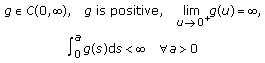 (1.7)
(1.7)or
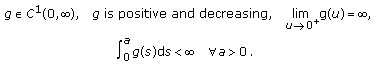 (1.8)
(1.8) -
(2)
Moreover, we compute solutions
 to the singular boundary value problem
  (1.9a)
 and the number and types of solutions to problem (1.6a)-(1.6b), provided that

 to the singular boundary value problem

and the singular problem (1.5a), (1.9b). Note that (1.9a) is the special case of (1.6a) with  satisfying (1.8).
In [4] similar questions in context of (1.6a) and the Dirichlet boundary conditions  ,
,  have been discussed. For further results on existence of positive and dead core solutions to differential equations of the types
  and
and  , we refer the reader to [5–9]. The Dirichlet conditions have been discussed in [5–7, 9], while [8] deals with the Robin conditions
  ,
,  ,
,  ,
,  .
.
We now recapitulate the main analytical results formulated in Theorems 2.10, 2.12, and 2.13. First, we introduce the auxiliary function

where  satisfies (1.7). By Lemma 2.2, the equation
  has a unique continuous solution
  , and the function

is continuous on  . Let
. Let  . Then the following statements hold.
-
(i)
Problem (1.6a)-(1.6b) has a positive solution if and only if

 . In addition, for each
  , problem (1.6a)-(1.6b) with
  has a unique positive solution such that
  ,
,  .
. -
(ii)
Problem (1.6a)-(1.6b) has a pseudo dead core solution if and only if
 (1.12)
This solution is unique.
-
(iii)
Problem (1.6a)-(1.6b) has a dead core solution if and only if
 (1.13)

 . In addition, for each
  , problem (1.6a)-(1.6b) with
  has a unique positive solution such that
  ,
,  .
.

In addition, for all such  , problem (1.6a)-(1.6b) has a unique dead core solution.
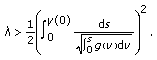
The final result concerning the multiplicity of positive solutions to problem (1.6a)-(1.6b) is given in Theorem 2.11. Let (1.8) hold and let 
 . Then
  and for each
  , there exist multiple positive solutions of problem (1.6a)-(1.6b).
In Section 2 analytical results are presented. Here, we formulate the existence and uniqueness results for the solutions of the boundary value problem (1.6a)-(1.6b) and study the dependance of the solution on the parameter values  . The numerical treatment of problems (1.9a)-(1.9b) and (1.5a)-(1.5b) based on the collocation method is discussed in Section 3, where for different values of
  , we study positive, pseudo dead core, and dead core solutions of problem (1.9a)-(1.9b) and positive solutions of problem (1.5a)-(1.5b).
2. Analytical Results
2.1. Auxiliary Functions
Let assumption (1.7) hold, and let us introduce auxiliary functions  , and
, and  as
as

where  ,
,


Here, the positive constants  and
and  are identical with those used in boundary conditions (1.6b). Note that the function
  is used in the analysis of positive and pseudo dead core solutions of problem (1.6a)-(1.6b), while the function
  for its dead core solutions.
Properties of  are described in the following lemma.
Lemma 2.1.
Let assumption (1.7) hold and let  . Then
  , and
, and  is increasing on
  .
.
Proof.
Let  be arbitrary,
  . Then
  , and
, and  is increasing on
  by [4, Lemma
  (where
  is replaced by
  )]. Since
  is arbitrary, the result immediately follows.
In the following lemma, we introduce functions  and
and  and discuss their properties.
Lemma 2.2.
Let assumption (1.7) hold. Then the following statements follow.
(i)The function  is continuous on
  , and
, and  for
for  .
.
(ii)For each  , there exists a unique
  such that

and  ,
,  for
for  ,
,  .
.
(iii)The function

is continuous on  .
.
Proof.
-
(i)
Let us define
 on
on  by
by 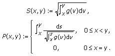 (2.6)
(2.6)
 on
on  by
by 
Then  . Let
. Let  and define
  . Then, by (1.7),
  . Hence

and consequently  , which means that
  is continuous at
  . Let
. Let  . We now show that
  is continuous at the point
  . Let us choose an arbitrary
  in the interval
  . Then
  for
for  and
and  , where

Since  by [4, Lemma
  (where 1 was replaced by
  )], it follows that
  is continuous at
  . The continuity of
  at
at  now follows from the fact that
  is continuous at this point. Hence
  is continuous on
  , and from
  we conclude
  . Since

we have  for
for  .
.
-
(ii)
Consider the equation
 , that is,
 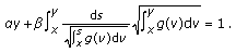 (2.10)
 , that is,
The function  is increasing on
  ,
,  , and, for
  ,
,  . Hence, for each
  , there exists a unique
  such that
  and
and  . Clearly,
  for
for  . In order to prove that
  , suppose the contrary, that is, suppose that
  is discontinuous at a point
  ,
,  . Then there exist sequences
  in
in  such that
  , and the sequences
  are convergent,
  ,
,  ,
,  . Let
. Let  in
in  and in
  . This means
  ,
,  , and
, and  by the definition of the function
  , which contradicts
  .
.
-
(iii)
By (ii),
 (2.11)

 and
and  for
for  . Hence, the function
  is continuous on
  and positive on
  . From

we now deduce that  . Since

where  , and
, and  on
on  ,
,  , we conclude
  . Hence
  is continuous at
  , and consequently
  .
.
Let  be the function from Lemma 2.2(ii) defined on the interval
  . From now on,
  denotes the value of
  at
at  , that is,

In the following lemma, we prove a property of  which is crucial for discussing multiple positive solutions of problem (1.6a)-(1.6b).
Lemma 2.3.
Let assumption (1.8) hold and let the function  be given by (2.5). Then there exists
  such that

Proof.
Note that  d
d . We deduce from [4, Lemma
  (with 1 replaced by
  )] that there exists an
  such that

If  for some
  , then (2.16) yields

Consequently, inequality (2.15) holds for such an  . If the statement of the lemma were false, then some
  would exist such that
  and
and

From the following equalities, compare (2.4),

and from  , we conclude that

Finally, from

we have  , which contradicts (2.18).
In order to discuss dead core solutions of problem (1.6a)-(1.6b) and their dead cores, we need to introduce two additional functions  and
and  related to
  and study their properties.
Lemma 2.4.
Assume that (1.7) holds and let  be given by (2.3). Then for each
  , there exists a unique
  such that

The function  is continuous and decreasing on
  , and the function

is continuous and increasing on  . Moreover,
  .
.
Proof.
It follows from (1.7) that  . Also,
  is increasing w.r.t. both variables,
  for any
  , and
, and  ,
,  for any
  . Hence, for each
  , there exists a unique
  such that
  . In order to prove that
  is decreasing on
  , assume on the contrary that
  for some
  . Then
  which contradicts
  for
for  . Hence,
  is decreasing on
  . If
. If  was discontinuous at a point
  , then there would exist sequences
  and
and  in
in  such that
  and
and  ,
,  are convergent,
  , and
, and  with
with  . Taking the limits
  in
in  and
and  , we obtain
  ,
,  . Consequently,
  by the definition of the function
  , which is not possible.
By (2.22),

and therefore,

It follows from the properties of  that the functions
  ,
,  are continuous, positive, and increasing on
  . Hence (2.25) implies that
  and
and  is increasing. Moreover,
  since
since  d
d is bounded on
  .
.
Corollary 2.5.
Let assumption (1.7) hold. Then

and for each  satisfying the inequality

there exists a unique  such that

Proof.
The equalities  for
for  and
and  imply that
  . Since the function
  defined by (2.23) is continuous and increasing on
  , it follows that
  for
for  ; see (2.26). Let us choose an arbitrary
  satisfying (2.27). Then
  . Now, the properties of
  guarantee that equation
  has a unique solution
  . This means that (2.28) holds for a unique
  .
.
2.2. Dependence of Solutions on the Parameter 

The following two lemmas characterize the dependence of positive and dead core solutions of problem (1.6a)-(1.6b) on the parameter  .
.
Lemma 2.6.
Let assumption (1.7) hold and let  be a positive solution of problem (1.6a)-(1.6b) for some
  . Also, let
  , and
, and  . Then
  ,
,  ,
,


where the function  is given by (2.2).
Proof.
Since  and
and  for
for  , we conclude that
  on
on  and
and  ,
,  . By integrating the equality
  over
over  , we obtain

and consequently, since  on
on  ,
,

Finally, integrating

over  yields (2.30). Now we set
  in (2.30) and obtain (2.29). Equality (2.31) follows from
  and from

Remark 2.7.
Let (1.7) hold and let  be a pseudo dead core solution of problem (1.6a)-(1.6b). Then, by the definition of pseudo dead core solutions,
  . We can proceed analogously to the proof of Lemma 2.6 in order to show that

where  , and
, and


From (2.38), we finally have  . Consequently,
  .
.
Remark 2.8.
If  , then
  ,
,  is the unique solution of problem (1.6a)-(1.6b). This solution is positive.
Lemma 2.9.
Let assumption (1.7) hold and let  be a dead core solution of problem (1.6a)-(1.6b) for some
  . Moreover, let
  . Then
  and there exists a point
  such that
  for
for  ,
,


where the function  is given by (2.3). Furthermore,
  is the unique dead core solution of problem (1.6a)-(1.6b) with
  .
.
Proof.
Since  is a dead core solution of problem (1.6a)-(1.6b) with
  , there exists by definition, a point
  such that
  ,
,  for
for  and
and  on
on  . Consequently,
  on
on  , and
, and  . We can now proceed analogously to the proof of Lemma 2.6 to show that

and (2.39) holds. Setting  in (2.39), we obtain (2.40). Also, from (1.6b),
  ,
,

equality (2.41) follows.
It remains to verify that  is the unique dead core solution of problem (1.6a)-(1.6b) with
  . Let us suppose that
  is another dead core solution of the above problem. Let
  for
for  and
and  on
on  for some
  . Then
  for
for  , and consequently
  on
on  and
and  . Hence, compare (2.40) and (2.41),


Since

by (2.41), and the function  is increasing and continuous on
  , we deduce from (2.45) and (2.46) that
  . Then (2.40) and (2.44) yield
  . Therefore,
  d
d for
for  . Finally, since
  for
for  and since by Lemma 2.1 the function
  is increasing on
  ,
,  follows. This completes the proof.
2.3. Main Results
Let the function  be given by (2.5) and let us denote by
  the range of the function
  restricted to the interval
  ,
,

Since  by Lemma 2.2(iii),
  for
for  and
and  , we can have either (i)
  for
for  , or (ii)
  for some
  . For (i), we have
  , while in case of (ii),
  with
with

holds. Clearly,  .
.
Positive solutions of problem (1.6a)-(1.6b) are analyzed in the following theorem.
Theorem 2.10.
Let assumption (1.7) hold. Then problem (1.6a)-(1.6b) has a positive solution if and only if 
 . Additionally, for each
  , problem (1.6a)-(1.6b) with
  has a unique positive solution
  such that
  and
and  .
.
Proof.
Let  be a positive solution of problem (1.6a)-(1.6b) for
  . By Lemma 2.6, (2.31) holds with
  and
and  . Furthermore, by Lemmas 2.2(ii) and 2.6,
  , which together with (2.29) implies that
  . Consequently,
 . For
. For  , problem (1.6a)-(1.6b) has the unique positive solution
  ; see Remark 2.8. Since
  ,
, 
 . Consequently, if problem (1.6a)-(1.6b) has a positive solution, then
 .
.
We now show that for each 
 , problem (1.6a)-(1.6b) has a positive solution, and if
  for some
  , then problem (1.6a)-(1.6b) has a unique positive solution
  such that
  and
and  . Let us choose
 . Then
  for some
  . If
. If  , then
  . Consequently,
  and
and  is the unique solution of problem (1.6a)-(1.6b). Clearly,
  and
and  since
since  . Let us suppose that
  . If
. If  is a positive solution of problem (1.6a)-(1.6b) and
  , then, by Lemma 2.6; see (2.30), the equality
  holds for
  , where
  is given by (2.1). Hence, in order to prove that for
  problem (1.6a)-(1.6b) has a unique positive solution
  such that
  and
and  , we have to show that the equation

has a unique solution  ; this solution is a positive solution of problem (1.6a)-(1.6b), and
  ,
,  . Since
  ,
,  is increasing by Lemma 2.1, and
  , (2.49) has a unique solution
  . It follows from
  and
and  that
that  and
and  . In addition,

Hence,  and
and  . In order to show that
  is continuous at
  , we set
  . Then, compare (2.49),

and therefore,

Consequently,  , and so
  is continuous at
  , or equivalently,
  . Now (2.50) indicates that
  and
and

Moreover, by the de L'Hospital rule,

As a result  and
and  for
for  . Since
  and, by (2.50),
  , we have

by Lemma 2.2(ii). Thus,  satisfies (1.6b), and therefore
  is a unique positive solution of problem (1.6a)-(1.6b) such that
  and
and  .
.
The following theorem deals with multiple positive solutions of problem (1.6a)-(1.6b).
Theorem 2.11.
Let assumption (1.8) hold. Then  , with
  given by (2.48), and for each
  , there exist multiple positive solutions of problem (1.6a)-(1.6b).
Proof.
By Lemmas 2.2(iii) and 2.3,  ,
,  , and
, and  in a right neighbourhood of
  . Hence,
  . Let us choose
  . Then there exist
  such that
  for
for  . Now Theorem 2.10 guarantees that problem (1.6a)-(1.6b) has positive solutions
  and
and  such that
  ,
,  . Since
  , we have
  and therefore, for each
  , problem (1.6a)-(1.6b) has multiple positive solutions.
Next, we present results for pseudo dead core solutions of problem (1.6a)-(1.6b). Note that here  .
.
Theorem 2.12.
Let assumption (1.7) hold. Then problem (1.6a)-(1.6b) has a pseudo dead core solution if and only if

Moreover, for  given by (2.56), problem (1.6a)-(1.6b) has a unique pseudo dead core solution such that
  .
.
Proof.
Let us assume that  is a pseudo dead core solution of problem (1.6a)-(1.6b) and let
  . Then, by Remark 2.7, equalities (2.36), (2.38) hold, and
  . Also, (2.37) implies that
  is a solution of the equation

where  and
and  are given by (2.1) and (2.56), respectively. The result follows by showing that equation (2.57) has a unique solution and that this solution is a pseudo dead core solution of problem (1.6a)-(1.6b). We verify these facts for solutions of (2.57) arguing as in the proof of Theorem 2.10, with
  replaced by 0.
In the final theorem below, we deal with dead core solutions of problem (1.6a)-(1.6b).
Theorem 2.13.
Let assumption (1.7) hold and let  be the function defined in Lemma 2.4. Then the following statements hold.
-
(i)
Problem (1.6a)-(1.6b) has a dead core solution if and only if
 (2.58)
 -
(ii)
For each
 satisfying (2.58), problem (1.6a)-(1.6b) has a unique dead core solution.
 -
(iii)
If the subinterval
 is the dead core of a dead core solution
  of problem (1.6a)-(1.6b), then
  and
and (2.59)

 satisfying (2.58), problem (1.6a)-(1.6b) has a unique dead core solution.
 is the dead core of a dead core solution
  of problem (1.6a)-(1.6b), then
  and
and
Proof.
-
(i)
Let
 be a dead core solution of problem (1.6a)-(1.6b) for some
  and let
  . Then there exists a point
  such that
  for
for  , and equalities (2.39), (2.40), and (2.41) are satisfied by Lemma 2.9. We deduce from (2.41) and from Lemma 2.4 that
  . Therefore, compare (2.40),
  (2.60)
 be a dead core solution of problem (1.6a)-(1.6b) for some
  and let
  . Then there exists a point
  such that
  for
for  , and equalities (2.39), (2.40), and (2.41) are satisfied by Lemma 2.9. We deduce from (2.41) and from Lemma 2.4 that
  . Therefore, compare (2.40),
Since

by Corollary 2.5, we have

Hence, if problem (1.6a)-(1.6b) has a dead core solution, then  satisfies inequality (2.58).
We now prove that for each  satisfying (2.58), problem (1.6a)-(1.6b) has a dead core solution. Let us choose
  satisfying (2.58). Then, by Corollary 2.5, there exists a unique
  such that

Let us now consider, compare (2.39),

where  is given by (2.1). Since
  and
and  is increasing on
  by Lemma 2.1,
  , and, by (2.63),
  , there exists a unique solution
  of (2.64) and
  ,
,  . In addition,

and consequently,  and
and  . Since

by the Mean Value Theorem for integrals, where  , we have

Therefore,

since  . Hence,
  is continuous at
  , and
, and  . Furthermore,

Let

Then  ,
,  for
for  ,
,  ,
,  , and
, and

Thus,

where  is given by (2.3). Since
  by Lemma 2.4,
  satisfies the boundary conditions (1.6b). Consequently,
  is a dead core solution of problem (1.6a)-(1.6b).
-
(ii)
Let us choose an arbitrary
 satisfying (2.58). By (i), problem (1.6a)-(1.6b) has a dead core solution which is unique by Lemma 2.9.
 -
(iii)
Let the subinterval
 be the dead core of a dead core solution
  of problem (1.6a)-(1.6b). Then, by Lemma 2.9, equalities (2.40) and (2.41) hold with
  replaced by
  and
and  . Since
  by the definition of the function
  , we have
  . Equality (2.59) now follows from (2.40) with
  and
and  replaced by
  and
and  , respectively.
 satisfying (2.58). By (i), problem (1.6a)-(1.6b) has a dead core solution which is unique by Lemma 2.9.
 be the dead core of a dead core solution
  of problem (1.6a)-(1.6b). Then, by Lemma 2.9, equalities (2.40) and (2.41) hold with
  replaced by
  and
and  . Since
  by the definition of the function
  , we have
  . Equality (2.59) now follows from (2.40) with
  and
and  replaced by
  and
and  , respectively.
Example 2.14.
We now turn to the case study of the boundary value problem (1.9a)-(1.9b),

Note that (1.9a)-(1.9b) is a special case of (1.6a)-(1.6b) with  satisfying (1.8). Since

we have

for  , and
, and  for
for  . By Lemma 2.2, the equation
  has a unique solution
  for
for  ,
,  ,
,  for
for  , and
, and  . Let
. Let

Then  ,
,  , and
, and  . In order to show that
  is increasing on
  it is sufficient to verify that
  is injective. Let us assume that this is not the case, then there exist
  ,
,  , such that
  . From
  ,
,  , or equivalently, from

it follows that  , and
, and  which is a contradiction. Hence,
  is increasing on
  and therefore, there exists the inverse function
  mapping
  onto
onto  . Since

and  for
for  , we have

Consequently,

In order to discuss the range  of the function
  and the value of
  for
for  , we first consider properties of the function

defined on  . Let
. Let

Then

where  . The function
  vanishes only at point

in the interval  , and
, and  , because
  and
and  . Since
  ,
,  on
on  ,
,  on
on  and
and

for  , we have
  on
on  and
and  on
on  . Let us define
  . Then
  , and it follows from
  that
that  on
on  and
and  on
on  . Consequently,
  is increasing on
  and decreasing on
  . It follows from the equality
  for
for  and from the properties of the functions
  and
and  that
that  is increasing on
  and decreasing on
  . Hence,
  , where
  . Also,

Using properties of the function  and the results of Theorems 2.10–2.13, we can now characterize the structure of the solution
  .
.
-
(i)
For each
 , there exists only a unique dead core solution of problem (1.9a)-(1.9b).
 -
(ii)
For
 , there exist a unique dead core solution and a unique positive solution of problem (1.9a)-(1.9b).
 -
(iii)
For each
 , there exist a unique dead core solution and exactly two positive solutions of problem (1.9a)-(1.9b).
 -
(iv)
For
 , there exist the unique pseudo dead core solution
  and a unique positive solution of problem (1.9a)-(1.9b).
 -
(v)
For each
 , there exist only a unique positive solution of problem (1.9a)-(1.9b).
 , there exists only a unique dead core solution of problem (1.9a)-(1.9b).
 , there exist a unique dead core solution and a unique positive solution of problem (1.9a)-(1.9b).
 , there exist a unique dead core solution and exactly two positive solutions of problem (1.9a)-(1.9b).
 , there exist the unique pseudo dead core solution
  and a unique positive solution of problem (1.9a)-(1.9b).
 , there exist only a unique positive solution of problem (1.9a)-(1.9b).
Using Theorem 2.10, Lemma 2.6, and the properties of the function  , we can specify further properties of positive solutions of problem (1.9a)-(1.9b).
-
(i)
If
 is the (unique) positive solution of problem (1.9a)-(1.9b) with
  , then
  , where
  is the root of the equation
  .
. -
(ii)
If
 are the (unique) positive solutions of problem (1.9a)-(1.9b) with
  , then
  ,
,  , where
  , are the roots of the equation
  .
.
 is the (unique) positive solution of problem (1.9a)-(1.9b) with
  , then
  , where
  is the root of the equation
  .
. are the (unique) positive solutions of problem (1.9a)-(1.9b) with
  , then
  ,
,  , where
  , are the roots of the equation
  .
.We are also able to give some more information on the dead core solutions of problem (1.9a)-(1.9b). Since

the function  ,
,  , is the solution of the equation
  . Let us choose an arbitrary
  . By Corollary 2.5, the equation; see (2.28),

has a unique solution  . Consequently,

One can easily show that the function

is the unique dead core solution of problem (1.9a)-(1.9b). Additionally, it follows from Theorem 2.13(iii) that  since
since  .
.
3. Numerical Treatment
We now aim at the numerical approximation to the solution of the following two-point boundary value problem:

For the numerical solution of (3.1), we are using the collocation method implemented in our Matlab code bvpsuite. It is a new version of the general purpose Matlab code sbvp, compare [10–12]. This code has already been used to treat a variety of problems relevant in application; see, for example, [13–17]. Collocation is a widely used and well-studied standard solution method for two-point boundary value problems, compare [18] and the references therein. It can also be successfully applied to boundary value problems with singularities.
In the scope of the code are systems of ordinary differential equations of arbitrary order. For simplicity of notation we present a problem of maximal order four which can be given in a fully implicit form,


In order to compute the numerical approximation, we first introduce a mesh

The approximation for  is a collocation function

where we require  in case that the order of the underlying differential equation is
  . Here,
  are polynomials of maximal degree
  which satisfy the system (3.2a) at
  inner collocation points

and the associated boundary conditions (3.2b).
Classical theory, compare [18], predicts that the convergence order for the global error of the method is at least  , where
  is the maximal stepsize,
  To increase efficiency, an adaptive mesh selection strategy based on an a posteriori estimate for the global error of the collocation solution is utilized. A more detailed description of the numerical approach can be found in [4].
The code bvpsuite also allows to follow a path in the parameter-solution space. This means that in the following problem setting, parameter  is unknown:


where  is given. The path following strategy can also cope with turning points in the path. The theoretical justification for the path following strategy implemented in bvpsuite has been given in [19].
We first study the boundary problem (1.9a)-(1.9b). Positive solutions of problem (1.5a)-(1.5b) will be discussed in Section 3.4.
The above analytical discussion indicates that depending on the values of  ,
,  ,
,  , the problem has one or more positive solutions, a pseudo dead core solution or a dead core solution. All numerical approximations have been calculated on a fixed mesh with
  subintervals and collocation degree
  . Figure 1 shows
  for our choice of parameters used in the following sections. Here,
  is given by (2.81).

 for
for  (a) and for
  ,
,  (b).
(b).
3.1. Positive Solutions
For  ),
),  , there exist a unique positive solution. This solution was found numerically by using the original problem formulation (1.9a)-(1.9b). For
  we obtain
  . In Figure 2 we display the numerical solution, the error estimate and the residual for
  . The residual
  is calculated by substituting the numerical solution
  into the differential equation,


Problem (1. 9a)-(1.9b): The numerical solution, the error estimate, and the residual for  ,
,  and
and  .
.
Due to the very small size of the error estimate and residual, it is obvious that the numerical approximation is very accurate. According to the analytical results, a solution to the problem satisfies  where
where  is a root of
  . Here, we have
  and
and  which again shows the high quality of the numerical solution. In Figure 3 we depict the results for the parameter
  ,
,  and
and  . For this choice of parameters
  and
and  .
.

Problem (1. 9a)-(1.9b): The numerical solution, the error estimate, and the residual for  ,
,  and
and  .
.
For  there exists a unique positive solution. To compute its numerical approximation, we rewrite the problem (1.9a)-(1.9b) and consider

The numerical results related to parameter sets  ,
,  , and
, and  ,
,  are shown in Figure 4 and Figure 5, respectively.

Problem (3. 8): The numerical solution, the error estimate, and the residual for  ,
,  and
and  .
.

Problem (3. 8): The numerical solution, the error estimate, and the residual for  ,
,  and
and  .
.
Again, the error estimate and the residual are both very small and  , so
, so  . Moreover, for the second set of parameters,
  and
and  .
.
For  with
with  there exist two positive solutions. These two different solutions for a fixed value of
  can be characterized via the roots
  of
of  for
for  . The choice of parameters remains the same. For
  ,
,  and
and  the solution corresponding to
  is shown in Figure 6. The solution corresponding to
  is depicted in Figure 7. Note that for these values of
  and
and  we have
  .
.

Problem (3. 8): The numerical solution, the error estimate, and the residual for  ,
,  and
and  . The associated root is
  .
.

Problem (3. 9): The numerical solution, the error estimate, and the residual for  ,
,  and
and  . The associated root is
  .
.
The first of those two solutions was found using the reformulated problem (3.8) with  as the right-hand side. For the second solution it was necessary to rewrite the problem again and use

with  as a free unknown parameter and
  as a necessary additional boundary condition. Here,
  and
and  . For comparison,
  and
and  . In Figures 8 and 9, two different positive solutions for the second parameter set,
  ,
,  , and
, and  , are shown. Note that
  ,
,  and
and  . For this example
  and
and  . Here,
  and
and  . Finally, for
  , there exists a unique positive solution. In Figures 10 and 11 we display the numerical results for
  ,
,  and for
  ,
,  , respectively. In this example,
  and
and  . Using this latter set of parameters, we obtain
  and
and  . All positive solutions could be easily found and they all show a very satisfactory level of accuracy.

Problem (3. 8): The numerical solution, the error estimate, and the residual for  ,
,  and
and  . The associated root is
  .
.

Problem (3. 9): The numerical solution, the error estimate, and the residual for  ,
,  and
and  . The associated root is
  .
.

Problem (3. 8): The numerical solution, the error estimate, and the residual for  ,
,  and
and  .
.

Problem (3. 8): The numerical solution, the error estimate, and the residual for  ,
,  and
and  .
.
3.2. Pseudo Dead Core Solutions
In order to calculate the pseudo dead core solutions, we solved the following problem:

where the differential equation has been premultiplied by the factor  . Otherwise, the problem formulated as (3.1) or (3.8), would have not been well defined at all points
  such that
  . In Figures 12 and 13, we report on the pseudo dead core solutions for


Problem (3. 10): The numerical solution, the error estimate, and the residual for  ,
,  and
and  .
.

Problem (3. 10): The numerical solution, the error estimate, and the residual for  ,
,  and
and  .
.
In this case, the analytical unique pseudo dead core solution is known,

Therefore, the exact global error is accessible. In Table 1, we show the values for the global error,  where
where  is the numerical solution at
  .
.
3.3. Dead Core Solutions
We now deal with the dead core solutions of the problem. Note that they only occur for

Moreover, the relation between  and
and  , where
  is such that the solution vanishes on
  , is given by

Also, the dead core solution is known,

For the experiments, we used  and
and  , in order to solve the problem,

Clearly, if we approached the problem (3.16) directly, we had to use the knowledge of  which is not available in general. Therefore, it is especially important to note that we were able to find the dead core solution without explicit knowledge of
  by treating the problem (3.10), formulated on the whole interval
  ,
,

instead of solving (3.16). In Figures 14 and 15, we report on the numerical test runs for  ,
,  , and two values of
  ,
,  and
and  , respectively. In Figures 16 and 17, analogous results for
  ,
,  , and
, and  ,
,  , respectively, can be found.

Problem (3. 10): The initial profile, the numerical solution, the error estimate, and the residual for  ,
,  and
and  .
.

Problem (3. 10): The initial profile, the numerical solution, the error estimate, and the residual for  ,
,  and
and  .
.

Problem (3. 10): The initial profile, the numerical solution, the error estimate, and the residual for  ,
,  and
and  .
.

Problem (3. 10): The initial profile, the numerical solution, the error estimate, and the residual for  ,
,  and
and  .
.
Table 2 contains the information on the exact global error of the numerical dead core solution. We report on its maximal value  for a wide range of parameters. Obviously, dead core solutions can be found without exact use of the known solution structure, but the initial profile must be chosen carefully to guarantee the Newton iteration to convergence.
3.4. Positive Solutions of Problem (1.5a)-(1.5b)
In this section, we deal with problem (1.5a)-(1.5b). Since this problem is very involved, we decided to simulate it numerically first in order to provide some preliminary information about its solution. The numerical treatment of (1.5a)-(1.5b) turned out to be not at all straightforward, but nevertheless, for a certain choice of parameters,  ,
,  ,
,  and
and  ,
,  , we were able to solve the problem and provide the error estimate and the residual for its approximative solution. We have applied the path following strategy implemented in bvpsuite to the boundary value problem

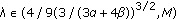
In Figures 19 to 28, we present numerical results for problem (3.18). The values of  for which we were able to calculate the associated numerical solutions, are shown in Figure 18. According to Figure 18, we have found a turning point at
  In a certain region below this value, there exist for any
  two different positive solutions.

Graph of the  path obtained in 76 steps of the path following procedure, where
  . The turning point has been found at
  .
.

Problem (3. 18): The numerical solution, the error estimate, and the residual for  .
.
In order to start the path following procedure we set  and used
  as an initial profile. For each further step, we used the solution from the previous step as an initial profile. The solution corresponding to the values of
  shown in Figures 19 and 20 is unique. For
  we have found two different positive solutions, compare Figures 21 and 22. Also, for
  , two different positive solutions exist; see Figures 23 and 24. Interestingly, solutions found in the vicinity of the turning point change rather fast, although the values of
  do not; see Figures 25 to 26. Finally, in the last step of the procedure, we obtained a solution which nearly reaches a pseudo dead core solution with
  .
.

Problem (3. 18): The numerical solution, the error estimate, and the residual for  .
.

Problem (3. 18): The numerical solution, the error estimate, and the residual for  .
.

Problem (3. 18): The numerical solution, the error estimate, and the residual for  .
.

Problem (3. 18): The numerical solution, the error estimate, and the residual for  .
.

Problem (3. 18): The numerical solution, the error estimate, and the residual for  .
.

Problem (3. 18): The numerical solution, the error estimate, and the residual for  .
.

Problem (3. 18): The numerical solution, the error estimate, and the residual for  .
.

Problem (3. 18): The numerical solution, the error estimate, and the residual for  .
.

Problem (3. 18): The numerical solution, the error estimate, and the residual for  .
.
References
Aris R: The Mathematical Theory of Diffusion and Reaction in Permeable Catalysts. Clarendon Press, Oxford, UK; 1975.
Baxley JV, Gersdorff GS: Singular reaction-diffusion boundary value problems. Journal of Differential Equations 1995,115(2):441-457. 10.1006/jdeq.1995.1022
Agarwal RP, O'Regan D, Staněk S:Dead core problems for singular equations with
 -Laplacian. Boundary Value Problems 2007, 2007:-16.
Staněk S, Pulverer G, Weinmüller EB: Analysis and numerical simulation of positive and dead-core solutions of singular two-point boundary value problems. Computers & Mathematics with Applications 2008,56(7):1820-1837. 10.1016/j.camwa.2008.03.029
Agarwal RP, O'Regan D, Staněk S:Positive and dead core solutions of singular Dirichlet boundary value problems with
 -Laplacian. Computers & Mathematics with Applications 2007,54(2):255-266. 10.1016/j.camwa.2006.12.026
Agarwal RP, O'Regan D, Staněk S:Dead cores of singular Dirichlet boundary value problems with
 -Laplacian. Applications of Mathematics 2008,53(4):381-399. 10.1007/s10492-008-0031-z
Bobisud LE: Asymptotic dead cores for reaction-diffusion equations. Journal of Mathematical Analysis and Applications 1990,147(1):249-262. 10.1016/0022-247X(90)90396-W
Bobisud LE: Behavior of solutions for a Robin problem. Journal of Differential Equations 1990,85(1):91-104. 10.1016/0022-0396(90)90090-C
Bobisud LE, O'Regan D, Royalty WD: Existence and nonexistence for a singular boundary value problem. Applicable Analysis 1988,28(4):245-256. 10.1080/00036818808839765
Auzinger W, Koch O, Weinmüller E: Efficient collocation schemes for singular boundary value problems. Numerical Algorithms 2002,31(1–4):5-25. 10.1023/A:1021151821275
Auzinger W, Kneisl G, Koch O, Weinmüller E: A collocation code for singular boundary value problems in ordinary differential equations. Numerical Algorithms 2003,33(1–4):27-39. 10.1023/A:1025531130904
Kitzhofer G: Numerical treatment of implicit singular BVPs, Ph.D. thesis. Institute for Analysis and Scientific Computing, Vienna University of Technology, Vienna, Austria;
Budd CJ, Koch O, Weinmüller E: Self-similar blow-up in nonlinear PDEs. Institute for Analysis and Scientific Computing, Vienna University of Technology, Vienna, Austria; 2004.
Budd CJ, Koch O, Weinmüller E: Computation of self-similar solution profiles for the nonlinear Schrödinger equation. Computing 2006,77(4):335-346. 10.1007/s00607-005-0157-8
Budd CJ, Koch O, Weinmüller E: Fron nonlinear PDEs to singular ODEs. Applied Numerical Mathematics 2006,56(3-4):413-422. 10.1016/j.apnum.2005.04.012
Kitzhofer G, Koch O, Lima P, Weinmüller E: Efficient numerical solution of the density profile equation in hydrodynamics. Journal of Scientific Computing 2007,32(3):411-424. 10.1007/s10915-007-9141-0
Rachůnková I, Koch O, Pulverer G, Weinmüller E: On a singular boundary value problem arising in the theory of shallow membrane caps. Journal of Mathematical Analysis and Applications 2007,332(1):523-541. 10.1016/j.jmaa.2006.10.006
Ascher UM, Mattheij RMM, Russell RD: Numerical Solution of Boundary Value Problems for Ordinary Differential Equations, Prentice Hall Series in Computational Mathematics. Prentice Hall, Englewood Cliffs, NJ, USA; 1988:xxiv+595.
Kitzhofer G, Koch O, Weinmüller EB: Pathfollowing for essentially singular boundary value problems with application to the complex Ginzburg-Landau equation. BIT. Numerical Mathematics 2009,49(1):141-160. 10.1007/s10543-008-0208-6
 -Laplacian. Boundary Value Problems 2007, 2007:-16.
 -Laplacian. Computers & Mathematics with Applications 2007,54(2):255-266. 10.1016/j.camwa.2006.12.026
 -Laplacian. Applications of Mathematics 2008,53(4):381-399. 10.1007/s10492-008-0031-z
Acknowledgments
This work was supported by the Austrian Science Fund Project P17253 and supported by Grant no. A100190703 of the Grant Agency of the Academy of Science of the Czech Republic and by the Council of Czech Government MSM 6198959214.
Author information
Authors and Affiliations
Corresponding author
Rights and permissions
Open Access This article is distributed under the terms of the Creative Commons Attribution 2.0 International License ( https://creativecommons.org/licenses/by/2.0 ), which permits unrestricted use, distribution, and reproduction in any medium, provided the original work is properly cited.
About this article
Cite this article
Pulverer, G., Staněk, S. & Weinmüller, E.B. Analysis and Numerical Solutions of Positive and Dead Core Solutions of Singular Sturm-Liouville Problems. Adv Differ Equ 2010, 969536 (2010). https://doi.org/10.1155/2010/969536
Received:
Accepted:
Published:
DOI: https://doi.org/10.1155/2010/969536