- Research Article
- Open access
- Published:
Existence Theorems for First-Order Equations on Time Scales with  -Carathéodory Functions
Advances in Difference Equations volume 2010, Article number: 650827 (2010)
Abstract
This paper concerns the existence of solutions for two kinds of systems of first-order equations on time scales. Existence results for these problems are obtained with new notions of solution tube adapted to these systems. We consider the general case where the right member of the system is  -Carathéodory and, hence, not necessarily continuous.
1. Introduction
In this paper, we establish existence results for the following systems:


Here,  is an arbitrary compact time scale where we note
  ,
,  , and
, and  . Moreover,
  is a
is a  -Carathéodory function and
  denotes one of the following boundary conditions:


In the literature, this kind of problem was mainly treated for  . The existence of extremal solutions was established in [1, 2]. Moreover, some existence results in the particular case where the time scale is a discrete set (difference equation) were obtained with the lower and upper solution method as in [3, 4]. In this paper, we introduce a new notion which generalizes to systems of first-order equations on time scales the notions of lower and upper solutions. This notion called solution tube for system (1.1) (resp., (1.2)) will be useful to get a new existence result for (1.1) (resp., (1.2)). Our notion of solution tube is in the spirit of the notion of solution tube for systems of first-order differential equations introduced in [5]. Our notion is new even in the case of systems of first-order difference equations. In this case, we generalize to the systems a result of [3] for equation (1.2).
Some papers treat the existence of solutions to systems of first-order equations on time scales. Existence results are obtained in [6, 7] under hypothesis different from ours. However, some particular cases obtained in [7] are corollaries of our existence result for problem (1.1). Also, our existence results treat the case where the right members in (1.1) and (1.2) are  -Carathéodory functions which are more general than continuous functions used for systems studied in [6, 7]. Let us mention that existence of extremal solutions for infinite systems of first-order equations of time scale with
  -Carathéodory functions is established in [8].
This paper is organized as follows. The third section presents an existence result for the problem (1.1), and in the last section, we obtain an existence theorem for the problem (1.2). We start with some notations, definitions, and results on time scales equations which are used throughout this paper.
2. Preliminaries and Notations
In this section, we establish notations, definitions, and results on equations on time scales which are used throughout this paper. The reader may consult [9–11] and the references therein to find the proofs and to get a complete introduction to this subject.
Let  be a time scale, which is a closed nonempty subset of
  . For
. For  , we define the forward jump operator
 (resp., the backward jump operator
 ) by
) by  (resp., by
  ). We suppose that
  if
if  is the maximum of
  and that
  if
if  is the minimum of
  . We say that
  is right-scattered (resp., left-scattered) if
  (resp., if
  ). We say that
  is isolated if it is right-scattered and left-scattered. Also, if
  and
and  , we say that
  is right-dense. If
  and
and  , we say that
  is left dense. Points that are right dense and left dense are called dense. The graininess function
 is defined by
  .
.
If  has a left-scattered maximum, then
  . Otherwise,
  . In summary,

If  is bounded, then
  where
where  .
.
Definition 2.1.
Assume  is a function and let
  . We say that
  is
is  -differentiable at
  if there exists a vector
  such that for all
  , there exists a neighborhood
  of
of  , where

for every  . We call
  the
the  -derivative of
  at
at  . If
. If  is
is  -differentiable at
  for every
  , then
  is called the
  -derivative of
  on
on  .
.
Theorem 2.2.
Assume  is a function and let
  . Then, we have the following.
-
(i)
If
 is
is  -differentiable at
  , then
  is continuous at
  .
. -
(ii)
If
 is continuous at
  and if
  is right-scattered, then
  is
is  -differentiable at
  and
and (2.3)
(2.3) -
(iii)
If
 is right dense, then
  is
is  -differentiable at
  if and only if
  exists in
  . In this case,
  .
. -
(iv)
If
 is
is  -differentiable at
  , then
  .
.
 is
is  -differentiable at
  , then
  is continuous at
  .
. is continuous at
  and if
  is right-scattered, then
  is
is  -differentiable at
  and
and
 is right dense, then
  is
is  -differentiable at
  if and only if
  exists in
  . In this case,
  .
. is
is  -differentiable at
  , then
  .
.Theorem 2.3.
If  are
are  -differentiable at
  , then
-
(i)
 is
is  -differentiable at
  and
and  ,
, -
(ii)
 is
is  -differentiable at
  for every
  and
and  ,
, -
(iii)
 is
is  -differentiable at
  and
and  ,
, -
(iv)
If
 , then
  is
is  -differentiable at
  and
and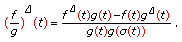 (2.4)
(2.4)
 is
is  -differentiable at
  and
and  ,
, is
is  -differentiable at
  for every
  and
and  ,
, is
is  -differentiable at
  and
and  ,
, , then
  is
is  -differentiable at
  and
and
The next result is an adaptation of Theorem 1.87 in [10].
Theorem 2.4.
Let  be an open set of
  and
and  a right-dense point. If
  is
is  -differentiable at
  and if
  is differentiable at
  , then
  is
is  -differentiable at
  and
and  .
.
Example 2.5.
Assume is
is - differentiable at
 . We know that
 is differentiable. If
 , by the previous theorem, we have
 .
.
Definition 2.6.
A function  is called
  -continuous provided it is continuous at right-dense points in
  and its left-sided limits exist (finite) at left-dense points in
  . The set of
  -continuous functions
  is denoted by
  . The set of functions
  that are
  -differentiable and whose
  -derivative is
  -continuous is denoted by
  .
.
It is possible to define a theory of measure and integration for an arbitrary bounded time scale  where
where  . We recall the notion of
  -measure as introduced in chapter 5 of [9]. Define
  the family of intervals of
  of the form

where  and
and  . The interval
  is understood as the empty set. An outer measure
  on
on  is defined as follows: for
  ,
,

Definition 2.7.
A set  is said to be
  -measurable if for every set
  ,
,

Now, denote

The Lebesgue -measure on
  , denoted by
  , is the restriction of
  to
to  . We get a complete measurable space with
  .
.
With this definition of complete measurable space for a bounded time scale  , we can define the notions of
  -measurability and
  -integrability for functions
  following the same ideas of the theory of Lebesgue integral. We omit here these definitions that an interested reader can find in [12]. We only present definitions and results which will be useful for this paper.
Definition 2.8.
Let  be a
be a  -measurable set and
  be a
be a  -measurable function. We say that
  provided

We say that a  -measurable function
  is in the set
  provided

for each of its components  .
.
Proposition 2.9.
Assume  . Then,

Many results of integration theory are established for measurable functions  where
where  is a complete measurable space. These results are in particular true for the measurable space
  . We recall two results of the theory of integration adapted to our situation.
Theorem 2.10 (Lebesgue-dominated convergence Theorem).
Let  be a sequence of functions in
  . If there exists a function
  such that
 -a.e.
-a.e.  and if there exists a function
  such that
 -a.e.
-a.e.  and for every
  , then
  in
in  .
.
Theorem 2.11.
The set  is a Banach space endowed with the norm
  .
.
The following results were obtained in [12] where a useful relation between the  -measure on
  (resp.,
  -integral on
  ) and the Lebesgue measure (
 ) on
) on  (resp., Lebesgue integral on
  ) is established. To establish these results, the authors of [12] prove that the set of right-scattered points of
  is at most countable. Then, there are a set of index
  and a set
  such that
  .
.
Proposition 2.12.
Let  . Then,
  is
is  -measurable if and only if
  is Lebesgue measurable. In such a case, the following properties hold for every
  -measurable set A.
-
(i)
If
 , then
 (2.12)
 -
(ii)
 if and only if
  and A has no right-scattered points. Here,
  .
.
 , then
 if and only if
  and A has no right-scattered points. Here,
  .
.To establish the relation between  -integration on
  and Lebesgue integration on a real compact interval, the function
  is extended to
  in the following way.

Theorem 2.13.
Let  be a
be a  -measurable set such that
  and let
  . Let
. Let  be a
be a  -measurable function and
  its extension on
  . Then,
  is
is  -integrable on
  if and only if
  is Lebesgue integrable on
  . In such a case, one has

Also, the function  can be extended on
  in another way. Define
  by
by

Definition 2.14.
A function  is said to be absolutely continuous on
 if for every
  , there exists a
  such that if
  with
with  is a finite pairwise disjoint family of subintervals of
  satisfying
  , then
  .
.
The three following results were obtained in [13].
Lemma 2.15.
If  is differentiable at
  , then
  is
is  -differentiable at
  and
and  .
.
Theorem 2.16.
Consider a function  and its extension
  . Then,
  is absolutely continuous on
  if and only if
  is absolutely continuous on
  .
.
Theorem 2.17.
A function  is absolutely continuous on
  if and only if
  is
is  -differentiable
  -almost everywhere on
  ,
,  and
and

We also recall the Banach Lemma.
Lemma 2.18.
Let  be a Banach space and
  an absolutely continuous function, then the measure of the set
  and
and  is zero.
Using the previous results, we now prove two propositions that will be used later.
Proposition 2.19.
Let  and
and  the function defined by

Then, 
 -almost everywhere on
  .
.
Proof.
By Theorem 2.13, remark that

We can also check that for  right scattered,

Obviously,

It is well known that  almost everywhere on
  . By Lemma 2.15, we have that
  except on a set
  such that
  . Since
  is continuous, for
  right scattered,

by Theorem 2.2(ii). Then,  is
is  -differentiable at
  . By Proposition 2.12(ii),
  and, then, the proposition is proved.
Proposition 2.20.
Let  be an absolutely continuous function, then the
  -measure of the set
  and
and  is zero.
Proof.
It suffices to consider the extension  of
of  on
on  and successively apply Theorem 2.16, Lemmas 2.18, 2.15, and the Proposition 2.12(ii).
We recall a notion of Sobolev's space of functions defined on a bounded time scale  where
where  . The definition and the result are from [14].
Definition 2.21.
We say that a function  belongs to
  if and only if
  and there exists a function
  such that
  and
and

with

We say that a function  is in the set
  if each of its components
  are in
  .
.
Theorem 2.22.
Suppose that  and that (2.22) holds for a function
  . Then, there exists a unique function
  absolutely continuous such that
  -almost everywhere on
  , one has
  and
and  . Moreover, if
  is
is  -continuous on
  , then there exists a unique function
  such that
  -almost everywhere on
  and such that
  on
on  .
.
By the previous theorem, we can conclude that  is also continuous.
Remark 2.23.
If , then its components
 are in
 . By Theorems 2.22 and 2.17,
 is
is - differentiable
 - a.e. on
 . From Example 2.5, we obtain
 - a.e. on
 .
.
We prove two maximum principles that will be useful to get a priori bounds for solutions of systems considered in this paper.
Lemma 2.24.
Let  such that
  -a.e.
-a.e.  . If one of the following conditions holds,
-
(i)
 ,
, -
(ii)
 ,
,
 ,
, ,
,then  , for every
  .
.
Proof.
Suppose the conclusion is false. Then, there exists  such that
  , since
  is continuous on
  . If
. If  , then
  exists, since
  and because
  . Then,

which is a contradiction since  . If
. If  , then there exists an interval
  such that
  for all
  . Thus,

by hypothesis and by Theorem 2.17. Hence, we get a contradiction. The case  is impossible if hypothesis (i) holds and if
  , we must have
  . If we take
  , by using previous steps of this proof, one can check that
  and, then, the lemma is proved.
Lemma 2.25.
Let  be a function such that
  -a.e. on
  if
if  , then
  , for every
  .
.
Proof.
If there exists  such that
  , then there exists a
  such that
  . If
. If  and
and  , then
  . Since
  ,
,  exists
  -almost everywhere. Then, we must have

which contradicts the hypothesis of the lemma. If  and
and  , there exists an interval
  such that
  for every
  . Then,

by Theorem 2.17, which contradicts the fact that  is a maximum. If
  , then by hypothesis, we must have
  . Thus, we can take
  , and by using the previous steps of this proof, one can check that
  . Then, the lemma is proved.
Definition 2.26.
For  , the exponential function
 may be defined as the unique solution of the initial value problem

More explicitly, the exponential function  is given by the formula

where for  , we define
  as
as

As direct consequences of Proposition 2.19 and Theorem 2.3, we get the following results.
Proposition 2.27.
If  , the function
  defined by

is a solution of the problem

Proposition 2.28.
If  , then the function
  defined by

is a solution of the problem

Proposition 2.29.
If  , then the function
  defined by

is a solution of the problem

We now define a notion of Carathéodory functions on a compact time scale.
Definition 2.30.
A function  is called a
  -Carathéodory function if the three following conditions hold.
-
(C-i)The map
 is
is  -measurable for every
  .
. -
(C-ii)The map
 is continuous
  -a.e.
-a.e.  .
. -
(C-iii)For every
 , there exists a function
  such that
  -a.e.
-a.e.  and for every
  such that
  .
.
 is
is  -measurable for every
  .
. is continuous
  -a.e.
-a.e.  .
. , there exists a function
  such that
  -a.e.
-a.e.  and for every
  such that
  .
.3. Existence Theorem for the Problem (1.1)
In this section, we establish an existence result for the problem (1.1). A solution of this problem will be a function  satisfying (1.1). Let us recall that
  is compact and
  . We introduce the notion of solution tube for the problem (1.1).
Definition 3.1.
Let  . We say that
  is a solution tube of (1.1) if
-
(i)

 -a.e.
-a.e.  and for every
  such that
  ,
, -
(ii)

 -a.e.
-a.e.  such that
  ,
, -
(iii)
 for every
  such that
  ,
, -
(iv)
If (BC) denotes (1.3),
 ; if (BC) denotes (1.4), then
  .
.

 -a.e.
-a.e.  and for every
  such that
  ,
,
 -a.e.
-a.e.  such that
  ,
, for every
  such that
  ,
, ; if (BC) denotes (1.4), then
  .
.We denote

If  is a real interval
  , our definition of solution tube is equivalent to the notion of solution tube introduced in [5].
We consider the following problem.

where

Let us define the operator  by
by

Proposition 3.2.
If  is a solution tube of (1.1), (1.3), then
  is compact.
Proof.
We first observe that from Definitions 2.30 and 3.1, there exists a function  such that
  -a.e.
-a.e.  for every
  .
.
Let  be a sequence of
  converging to
  . By Proposition 2.9,

where  .
.
Then, we must show that the sequence  defined by

converges to the function  in
in  where
where

We can easily check that  for every
  and, then, by (C-ii) of Definition 2.30,
  -a.e.
-a.e.  . Using also the fact that
 -a.e.
-a.e.  , we deduce that
  in
in  by Theorem 2.10. This prove the continuity of
  .
.
For the second part of the proof, we have to show that the set  is relatively compact. Let
  . Therefore,

So,  is uniformly bounded. This set is also equicontinuous since for every
  ,
,

By an analogous version of the Arzelà-Ascoli Theorem adapted to our context,  is relatively compact. Hence,
  is compact.
We now define the operator  by
by

The following result can be proved as the previous one.
Proposition 3.3.
If  is a solution tube of (1.1), (1.4), then the operator
  is compact.
Now, we can obtain the main theorem of this section.
Theorem 3.4.
If  is a solution tube of (1.1), then the problem (1.1) has a solution
  .
.
Proof.
By Proposition 3.2 (resp., Proposition 3.3),  (resp.,
  ) is compact. It has a fixed point by the Schauder fixed-point Theorem. Proposition 2.27 (resp., Proposition 2.28) implies that this fixed point is a solution for the problem (3.2). Then, it suffices to show that for every solution
  of (3.2),
  .
.
Consider the set  . By Remark 2.23,
  -a.e. on the set
  , we have

If  is right scattered, then
  and
and

Therefore, since  is a solution tube of (1.1), we have
  -a.e. on
  that
that

On the other hand, we have  -a.e. on
  that
that

This last equality follows from Definition 3.1(iii) and Proposition 2.20.
If we set  , then
  -almost everywhere on
  . Moreover, since
  is a solution tube of (1.1) and
  satisfies (1.3) (resp.,
  satisfies (1.4)), then
  (resp.,
  ). Lemma 2.24 implies that
  . Therefore,
  and, hence, the theorem is proved.
Existence theorems are obtained in [7] for the problem (1.1), (1.3) when  is continuous by using a hypothesis different of ours. When
  is bounded, we can directly use the Schauder fixed-point Theorem to deduce the existence of a solution to (1.1), (1.3). We now show that in the case where
  is unbounded, Theorems 4.7 and 4.8 of [7] become corollaries of our existence theorem.
Corollary 3.5.
Let  be an unbounded continuous function. If there exist non-negative constants
  and
and  such that

for every  and every
  , then the problem (1.1), (1.3) has at least one solution.
Proof.
Observe that  since
since  is unbounded. By hypothesis, there exists a constant
  such that
  . Let us define
  by
by

Then,  for every
  and, thus,

for every  and every
  . Then, if we take
  , we get a solution tube
  for our problem and by Theorem 3.4, the problem has a solution
  such that
  for every
  .
.
Corollary 3.6.
Let  be an unbounded continuous function. If there exists a nonnegative constant
  such that

for every  and every
  , then the problem (1.1), (1.3) has at least one solution.
4. Existence Theorem for the Problem (1.2)
In this section, we establish an existence result for the problem (1.2). A solution of this problem will be a function  for which (1.2) is satisfied. As before,
  is compact and
  . We introduce the notion of solution tube for the problem (1.2). Conditions of this definition are slightly different than conditions in Definition 3.1.
Definition 4.1.
Let  . We say that
  is a solution tube of (1.2) if
-
(i)
 -a.e.
-a.e.  and for every
  such that
  ,
, -
(ii)
 and
and  ,
,  -a.e.
-a.e.  such that
  ,
, -
(iii)
 .
.
 -a.e.
-a.e.  and for every
  such that
  ,
, and
and  ,
,  -a.e.
-a.e.  such that
  ,
, .
.We consider the following problem.

where  is defined in (3.3).
Let us define the operator  by
by

The following result can be proved as Proposition 3.2.
Proposition 4.2.
If  is a solution tube of (1.2), then the operator
  is compact.
Here is the main existence theorem for problem (1.2).
Theorem 4.3.
If  is a solution tube of (1.2), then the problem (1.2) has a solution
  .
.
Proof.
By Proposition 4.2,  is compact. Then, by the Schauder fixed-point Theorem,
  has a fixed point which is a solution of (4.1) by Proposition 2.29. It suffices to show that for every solution
  of (4.1),
  .
.
Let us consider the set  . By Remark 2.23,
  -a.e. on the set
  we have

If  is right scattered, then
  and
and

Since  is a solution tube of (1.2), we have
  -a.e. on
  that
that

On the other hand, we have  -a.e. on
  that
that

If we set  , then
  -almost everywhere on
  . Moreover, since
  is a solution tube of (1.2) and
  satisfies (1.4),
  . Lemma 2.25 implies that
  . So,
. So,  and the theorem is proved.
Let us observe that the following results obtained in [6] and [15], respectively, are different from ours.
Theorem 4.4.
Let  be a continuous function with
  such that
  . If there exist nonnegative constants
  and
and  such that

for every  , where
  is defined by
  with
with

then the problem (1.2) has a solution.
Theorem 4.5.
Let  ,
,  and
and  a continuous function. If there exist nonnegative constants
  and
and  such that

for every  , then the difference equation (1.2) has one solution.
Observe that Theorem 4.3 is valid for every arbitrary time scale  . Here is an example where (4.7) and (4.9) are not satisfied, but where Theorem 4.3 can be applied to deduce the existence of a solution.
Example 4.6.
Consider the system

where  are real positive constants such that
  and where
  is a continuous function such that
  for every
  .
.
We first show that this system do not satisfy (4.7). Suppose there exist non-negative constants  and
and  such that

for every  .
.
If we define  , then

for every  .
.
Then,

for every  , where
  ,
,  ,
,  , and
, and  . Taking the limit as
  , we get a contradiction. Similarly, if
  , it can be shown that (4.9) is not satisfied. On the other hand, it is easy to verify that
  is a solution tube of (4.10). By Theorem 4.3, this problem has a solution
  such that
  for every
  .
.
Definition 4.1 generalizes the notions of lower and upper solutions  and
and  introduced in [3] in the particular case where the problem (1.2) is considered with
  ,
,  for some
  and with
  depending only on
  . We recall these definitions. Consider the problem

where  .
.
Definition 4.7.
A vector  (resp.,
  ) is called an upper solution (resp., a lower solution) of (4.14) if
-
(i)
for every
 ,
,  (resp.,
  ),
), -
(ii)
 (resp.,
  ).
).
 ,
,  (resp.,
  ),
), (resp.,
  ).
).Remark that if  are, respectively, lower and upper solutions of (4.14) such that
  for every
  , then
  is a solution tube for this problem. Conversely, if
  is a solution tube of (4.14), then
  and
and  are, respectively, lower and upper solution for the same problem if, in addition, condition (ii) of Definition 4.7 is satisfied. Then, Theorem 5 of [3] becomes a corollary of Theorem 4.3.
Corollary 4.8.
If  are, respectively, lower and upper solutions of (4.14) such that
  for every
  , then this equation has a solution
  such that
  for every
  .
.
References
Otero-Espinar V, Vivero DR: Existence of extremal solutions by approximation to a first-order initial dynamic equation with Carathéodory's conditions and discontinuous non-linearities. Journal of Difference Equations and Applications 2006,12(12):1225-1241. 10.1080/10236190600949808
Otero-Espinar V, Vivero DR: The existence and approximation of extremal solutions to several first-order discontinuous dynamic equations with nonlinear boundary value conditions. Nonlinear Analysis: Theory, Methods & Applications 2008,68(7):2027-2037. 10.1016/j.na.2007.01.030
Bereanu C, Mawhin J: Existence and multiplicity results for periodic solutions of nonlinear difference equations. Journal of Difference Equations and Applications 2006,12(7):677-695. 10.1080/10236190600654689
Franco D, O'Regan D, Perán J: Upper and lower solution theory for first and second order difference equations. Dynamic Systems and Applications 2004,13(2):273-282.
Mirandette B: Résultats d'Existence pour des Systèmes d'Équations Différentielles du Premier Ordre avec Tube-Solution. Mémoire de Maîtrise, Université de Montréal, Montréal, Canada; 1996.
Dai Q, Tisdell CC: Existence of solutions to first-order dynamic boundary value problems. International Journal of Difference Equations 2006,1(1):1-17.
Tisdell CC, Zaidi A: Basic qualitative and quantitative results for solutions to nonlinear, dynamic equations on time scales with an application to economic modelling. Nonlinear Analysis: Theory, Methods & Applications 2008,68(11):3504-3524. 10.1016/j.na.2007.03.043
Otero-Espinar V, Vivero DR: Existence and approximation of extremal solutions to first-order infinite systems of functional dynamic equations. Journal of Mathematical Analysis and Applications 2008,339(1):590-597. 10.1016/j.jmaa.2007.06.031
Bohner M, Peterson A: Advances in Dynamic Equations on Time Scales. Birkhäuser, Boston, Mass, USA; 2003:xii+348.
Bohner M, Peterson A: Dynamic Equations on Time Scales. Birkhäuser, Boston, Mass, USA; 2001:x+358.
Hilger S: Analysis on measure chains—a unified approach to continuous and discrete calculus. Results in Mathematics. Resultate der Mathematik 1990,18(1-2):18-56.
Cabada A, Vivero DR:Expression of the Lebesgue
 -integral on time scales as a usual Lebesgue integral: application to the calculus of
  -antiderivatives. Mathematical and Computer Modelling 2006,43(1-2):194-207. 10.1016/j.mcm.2005.09.028
Cabada A, Vivero DR: Criterions for absolute continuity on time scales. Journal of Difference Equations and Applications 2005,11(11):1013-1028. 10.1080/10236190500272830
Agarwal RP, Otero-Espinar V, Perera K, Vivero DR: Basic properties of Sobolev's spaces on time scales. Advances in Difference Equations 2006, 2006:-14.
Tisdell CC: On first-order discrete boundary value problems. Journal of Difference Equations and Applications 2006,12(12):1213-1223. 10.1080/10236190600949790
 -integral on time scales as a usual Lebesgue integral: application to the calculus of
  -antiderivatives. Mathematical and Computer Modelling 2006,43(1-2):194-207. 10.1016/j.mcm.2005.09.028
Acknowledgment
The author would like to thank Professor Marlene Frigon for useful discussion and comments and the FQRNT for financial support.
Author information
Authors and Affiliations
Corresponding author
Rights and permissions
Open Access This article is distributed under the terms of the Creative Commons Attribution 2.0 International License (https://creativecommons.org/licenses/by/2.0), which permits unrestricted use, distribution, and reproduction in any medium, provided the original work is properly cited.
About this article
Cite this article
Gilbert, H. Existence Theorems for First-Order Equations on Time Scales with  -Carathéodory Functions.
Adv Differ Equ 2010, 650827 (2010). https://doi.org/10.1155/2010/650827
-Carathéodory Functions.
Adv Differ Equ 2010, 650827 (2010). https://doi.org/10.1155/2010/650827
Received:
Accepted:
Published:
DOI: https://doi.org/10.1155/2010/650827